The Array Structure

The array is probably the most widely known structure of data because in many languages, including FORTRAN and ALGOL 60, it is the only explicitly available structure. An array is a homogeneous structure; it consists of components which are all of the same type, called the base type. The array is also a so-called random-access structure; all components can be selected at random and are equally accessible. In order to denote an individual component, the name of the entire structure is augmented by the so-called index selecting the component. This index is to be a value of the type defined as the index type of the array. The definition of an array type $T$ therefore specifies both a base type $T_0$ and an index type $I$ .

type T = array[I] of T₀

(1.10)

Examples

type Row  = array[1 .. 5] of real
type Card = array[1 .. 80] of char
type alfa = array[1 .. 10] of char

12 A particular value of a variable

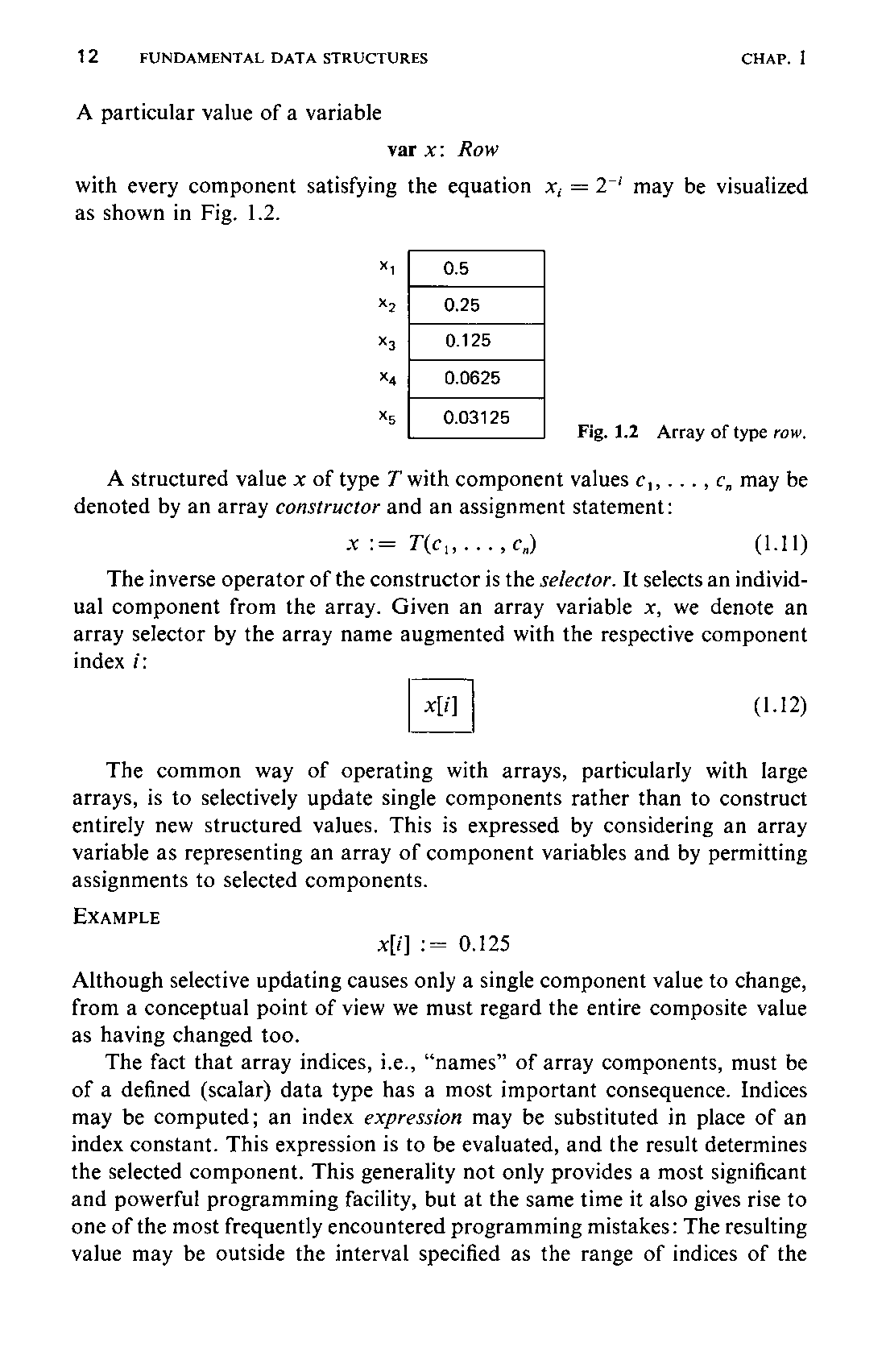
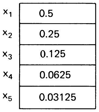
var x: Row

with every component satisfying the equation $x_i = 2^{-i}$ may be visualized as shown in Fig. 1.2.

Fig. 1.2 Array of type row. — **Fig. 1.2** Array of type row.

A structured value $x$ of type $T$ with component values $c_1, \ldots, c_n$ may be denoted by an array constructor and an assignment statement:

x := T(c₁, ..., cₙ)

(1.11)

The inverse operator of the constructor is the selector. It selects an individual component from the array. Given an array variable $x$ , we denote an array selector by the array name augmented with the respective component index $i$ :

x[i]

(1.12)

The common way of operating with arrays, particularly with large arrays, is to selectively update single components rather than to construct entirely new structured values. This is expressed by considering an array variable as representing an array of component variables and by permitting assignments to selected components.

Example

x[i] := 0.125

Although selective updating causes only a single component value to change, from a conceptual point of view we must regard the entire composite value as having changed too.

The fact that array indices, i.e., “names” of array components, must be of a defined (scalar) data type has a most important consequence. Indices may be computed; an index expression may be substituted in place of an index constant. This expression is to be evaluated, and the result determines the selected component. This generality not only provides a most significant and powerful programming facility, but at the same time it also gives rise to one of the most frequently encountered programming mistakes: The resulting value may be outside the interval specified as the range of indices of the13 array. We will assume that adequate computing systems provide a warning in the case of such a mistaken access to a non-existent array component.

Normally, an index type will have to be a scalar type, i.e., an unstructured type upon which an ordering relation is defined. If the base type of an array is also an ordered type, then a natural ordering relation is given upon that array type. The natural ordering of two arrays is determined by the two corresponding unequal components with least indices. This is expressed formally as follows:

Given two arrays $x$ and $y$ , the relation $x < y$ holds if and only if there exists an index $k$ such that $x[k] < y[k]$ and $x[i] = y[i]$ for all $i < k$ . (1.13)

For example,

\begin{gathered} (2, 3, 5, 7, 9) < (2, 3, 5, 7, 11) \\ \text{‘LABEL’} < \text{‘LIBEL’} \end{gathered}

In most applications, however, no ordering is presumed to exist on array types.

The cardinality of a structured type is the product of the cardinality of its components. Since all components of an array type $A$ are of the same base type $B$ , we obtain

\text{cardinality}(A) = (\text{cardinality}(B))^n \tag{1.14}

where $n = \text{cardinality}(I)$ , and $I$ is the array’s index type.

The following short piece of program shows the use of the array selector. The purpose of the program is to find the least index $i$ of a component with value $x$ . The search is performed by a sequential scan of the array $a$ , declared as

var a: array [1 .. N] of T;  {N>0}
i := 0;
repeat i := i+1 until (a[i]=x) ∨ (i=N);
if a[i] ≠ x then “there is no such element in a”

(1.15)

A variant of this program uses the common technique of a sentinel posted at the end of the array. The purpose of the sentinel is to allow a simplification of the termination condition of the repetition.

var a: array[1 .. N+1] of T;
i := 0; a[N+1] := x;
repeat i := i+1 until a[i] = x;
if i > N then “there is no such element in a”

(1.16)

The assignment a[N+1] := x is an example of selective updating, i.e., of the alteration of a selected component of a structured variable. The essential condition that holds no matter how often the statement i := i+1 was repeated, is

a[j] \ne x, \qquad \text{for } j = 1 \ldots i-1

14in both versions (1.15) and (1.16). This condition is therefore called a loop invariant.

The search can, of course, be speeded up considerably if the elements are already ordered (sorted). In this case, the principle of repeated halving of the interval in which the desired element must be searched is most common. It is called bisection or binary search and is shown in (1.17). In each repetition, the inspected interval between indices $i$ and $j$ is bisected. The number of required comparisons is therefore at most $[\log_2 (N)]$ .

i := 1; j := N;
repeat k := (i+j) div 2;
  if x > a[k] then i := k+1 else j := k-1
until (a[k]=x) ∨ (i>j)

(1.17)

(The relevant invariant condition at the entrance of the repeat statement is

\begin{aligned} a[h] &< x \qquad \text{for} \quad h = 1 \ldots i-1 \\ a[h] &\ge x \qquad \text{for} \quad h = j+1 \ldots N \end{aligned}

Hence, if the program terminates with $a[k] \ne x$ , it implies that there exists no $a[h] = x$ with $1 \le h \le N$ .)

Constituents of array types may themselves be structured. An array variable whose components are again arrays is called a matrix. For example,

M: array[1 .. 10] of Row

is an array consisting of ten components (rows), each consisting of five components of type real, and is called a $10 \times 5$ matrix with real components. Selectors may be concatenated accordingly, such that

M[i][j]

denotes the $j$ th component of row M[i], which is the $i$ th component of $M$ . This is usually abbreviated as

M[i,j]

and in the same spirit the declaration

M: array[1 .. 10] of array[1 .. 5] of real

can be written more concisely as

M: array[1 .. 10, 1 .. 5] of real.

If a certain operation has to be performed on all components of an array or on adjacent components of a part of the array, then this fact may conveniently be emphasized by using the for statement, as shown in the following example.

Assume that a fraction $f$ is represented by the array $d$ such that

f = \sum_{i=1}^{k-1} d_i * 10^{-i}

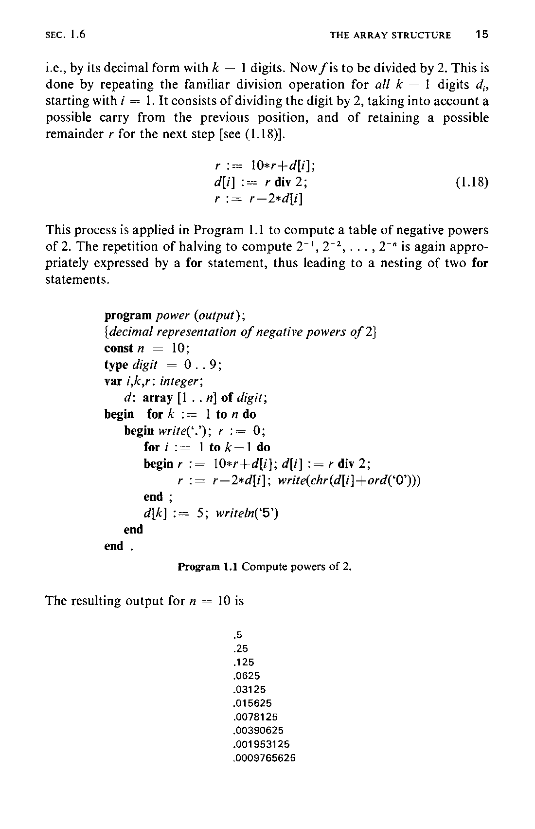
15i.e., by its decimal form with $k-1$ digits. Now $f$ is to be divided by 2. This is done by repeating the familiar division operation for all $k-1$ digits $d_i$ , starting with $i = 1$ . It consists of dividing the digit by 2, taking into account a possible carry from the previous position, and of retaining a possible remainder $r$ for the next step [see (1.18)].

r := 10*r+d[i];
d[i] := r div 2;
r := r-2*d[i]

(1.18)

This process is applied in Program 1.1 to compute a table of negative powers of 2. The repetition of halving to compute $2^{-1}, 2^{-2}, \ldots, 2^{-n}$ is again appropriately expressed by a for statement, thus leading to a nesting of two for statements.

program power (output);
{decimal representation of negative powers of 2}
const n = 10;
type digit = 0 .. 9;
var i,k,r: integer;
    d: array [1 .. n] of digit;
begin for k := 1 to n do
   begin write(‘.’); r := 0;
      for i := 1 to k-1 do
      begin r := 10*r+d[i]; d[i] := r div 2;
            r := r-2*d[i]; write(chr(d[i]+ord(‘0’)))
      end ;
      d[k] := 5; writeln(‘5’)
   end
end .

Program 1.1 Compute powers of 2.

The resulting output for $n = 10$ is

.5
.25
.125
.0625
.03125
.015625
.0078125
.00390625
.001953125
.0009765625