Introduction

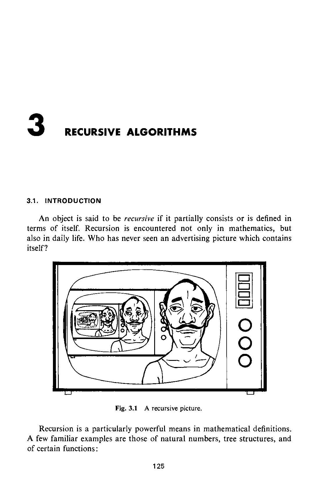
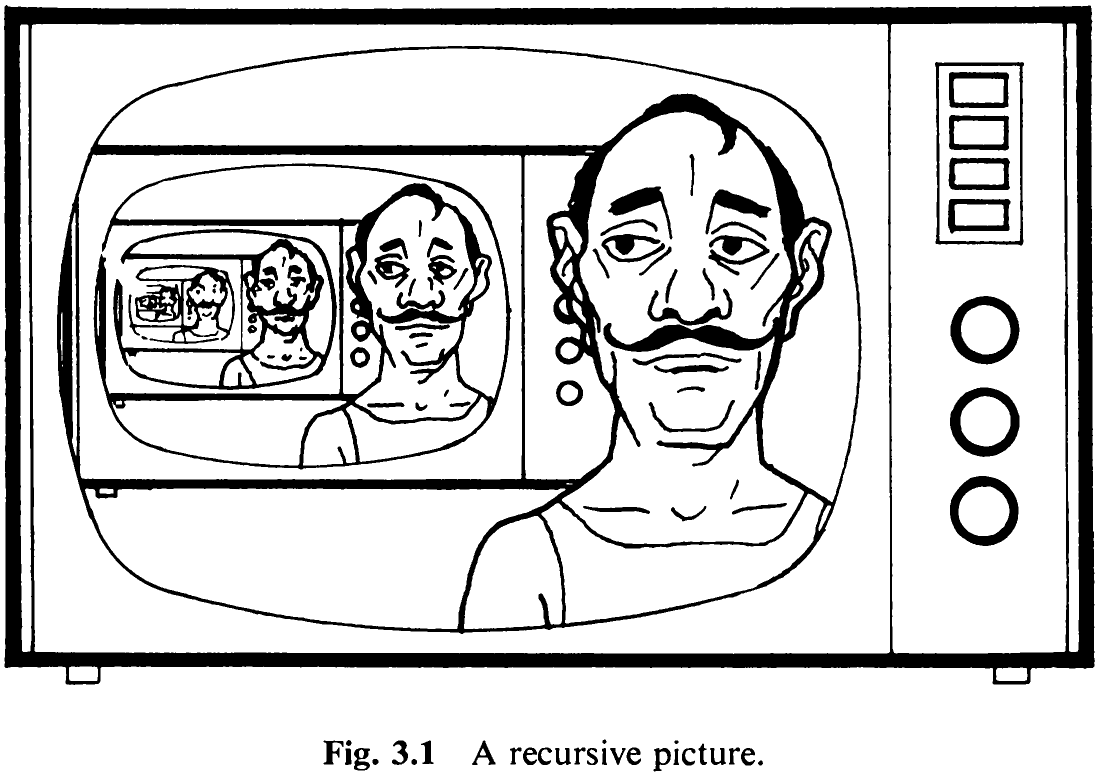
An object is said to be recursive if it partially consists or is defined in terms of itself. Recursion is encountered not only in mathematics, but also in daily life. Who has never seen an advertising picture which contains itself?

Recursion is a particularly powerful means in mathematical definitions. A few familiar examples are those of natural numbers, tree structures, and of certain functions:

1. Natural numbers:

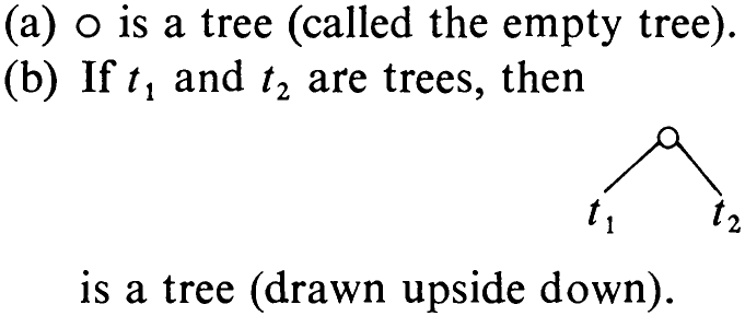
2. Tree structures

3. The factorial function ! (for non-negative integers):

The power of recursion evidently lies in the possibility of defining an infinite set of objects by a finite statement. In the same manner, an infinite number of computations can be described by a finite recursive program, even if this program contains no explicit repetitions. Recursive algorithms, however, are primarily appropriate when the problem to be solved, or the function to be computed, or the data structure to be processed are already defined in recursive terms. In general, a recursive progtam can be expressed as a composition @ of base statements S, (not containing P) and P itself.

The necessary and sufficient tool for expressing programs recursively is the procedure or subroutine, for it allows a statement to be given a name by which this statement may be invoked. If a procedure P contains an explicit reference to itself, then it is said to be directly recursive; if P contains a reference to another procedure Q which contains a (direct or indirect) reference to P, then P is said to be indirectly recursive. The use of recursion may therefore not be immediately apparent from the program text.

It is common to associate a set of local objects with a procedure, i.e., a set of variables, constants, types, and procedures which are defined locally to this procedure and have no existence or meaning outside this procedure. Each time such a procedure is activated recursively, a new set of local, bound variables is created. Although they have the same names as their corresponding elements in the set local to the previous instance of the procedure, their values are distinct, and any conflict in naming is avoided by the rules of scope of identifiers: the identifiers always refer to the most recently created set of variables. The same rule holds for procedure parameters which by definition are bound to the procedure.

Like repetitive statements, recursive procedures introduce the possibility of non-terminating computations, and thereby also the necessity of considering127 the problem of termination. A fundamental requirement is evidently that the recursive call of a procedure P is subjected to a condition B, which at some time becomes non-satisfied. The scheme for recursive algorithms may therefore be expressed more precisely as

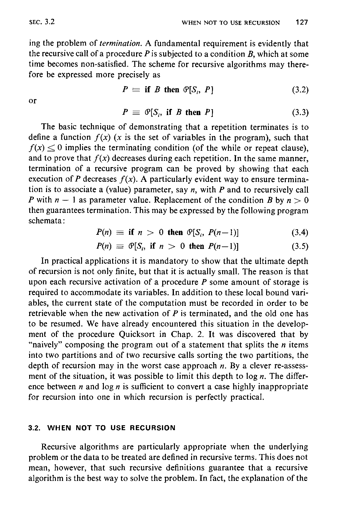
The basic technique of demonstrating that a repetition terminates is to define a function f(x) (x is the set of variables in the program), such that F(x) <0 implies the terminating condition (of the while or repeat clause), and to prove that f(x) decreases during each repetition. In the same manner, termination of a recursive program can be proved by showing that each execution of P decreases f(x). A particularly evident way to ensure termination is to associate a (value) parameter, say 1, with P and to recursively call P with n — | as parameter value. Replacement of the condition B by n > 0 then guarantees termination. This may be expressed by the following program schemata:

In practical applications it is mandatory to show that the ultimate depth of recursion is not only finite, but that it is actually small. The reason is that upon each recursive activation of a procedure P some amount of storage is required to accommodate its variables. In addition to these local bound variables, the current state of the computation must be recorded in order to be retrievable when the new activation of P is terminated, and the old one has to be resumed. We have already encountered this situation in the development of the procedure Quicksort in Chap. 2. It was discovered that by “naively” composing the program out of a statement that splits the n items into two partitions and of two recursive calls sorting the two partitions, the depth of recursion may in the worst case approach n. By a clever re-assessment of the situation, it was possible to limit this depth to log n. The difference between x and log n is sufficient to convert a case highly inappropriate for recursion into one in which recursion is perfectly practical.