The Optimal Selection Problem

The last example of a backtracking algorithm is a logical extension of the previous two examples represented by the general schema (3.35). First we were using the principle of backtracking to find a single solution to a given problem. This was exemplified by the knight’s tour and the eight queens. Then we tackled the goal of finding a// solutions to a given problem; the examples were those of the eight queens and the stable marriages. Now we wish to find the optimal solution.

To this end, it is necessary to generate all possible solutions, and in the155 course of generating them to retain the one which is optimal in some specific sense. Assuming that optimality is defined in terms of some positive valued function f(s), the algorithm is derived from schema (3.35) by replacing the statement print solution by the statement

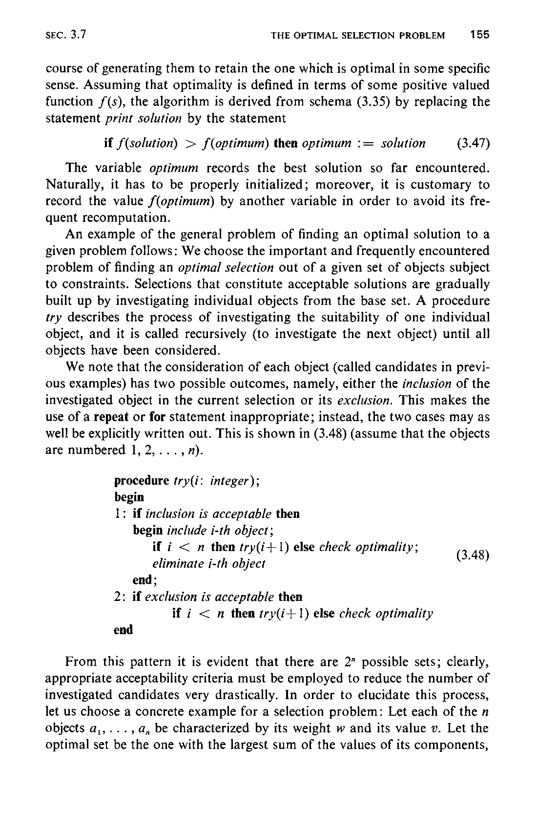
The variable optimum records the best solution so far encountered. Naturally, it has to be properly initialized; moreover, it is customary to record the value f(optimum) by another variable in order to avoid its frequent recomputation.

An example of the general problem of finding an optimal solution to a given problem follows: We choose the important and frequently encountered problem of finding an optimal selection out of a given set of objects subject to constraints. Selections that constitute acceptable solutions are gradually built up by investigating individual objects from the base set. A procedure try describes the process of investigating the suitability of one individual object, and it is called recursively (to investigate the next object) until all objects have been considered.

We note that the consideration of each object (called candidates in previous examples) has two possible outcomes, namely, either the inclusion of the investigated object in the current selection or its exclusion. This makes the use of a repeat or for statement inappropriate; instead, the two cases may as well be explicitly written out. This is shown in (3.48) (assume that the objects are numbered 1, 2,..., 7).

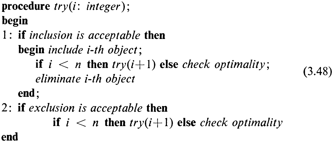
From this pattern it is evident that there are 2” possible sets; clearly, appropriate acceptability criteria must be employed to reduce the number of investigated candidates very drastically. In order to elucidate this process, let us choose a concrete example for a selection problem: Let each of the n objects a,,..., a, be characterized by its weight w and its value v. Let the optimal set be the one with the largest sum of the values of its components,156 and let the constraint be a limit on the sum of their weight. This is a problem well-known to all travellers who pack suitcases by selecting from n items in such a way that their total value is optimal and that their total weight does not exceed a specific allowance.

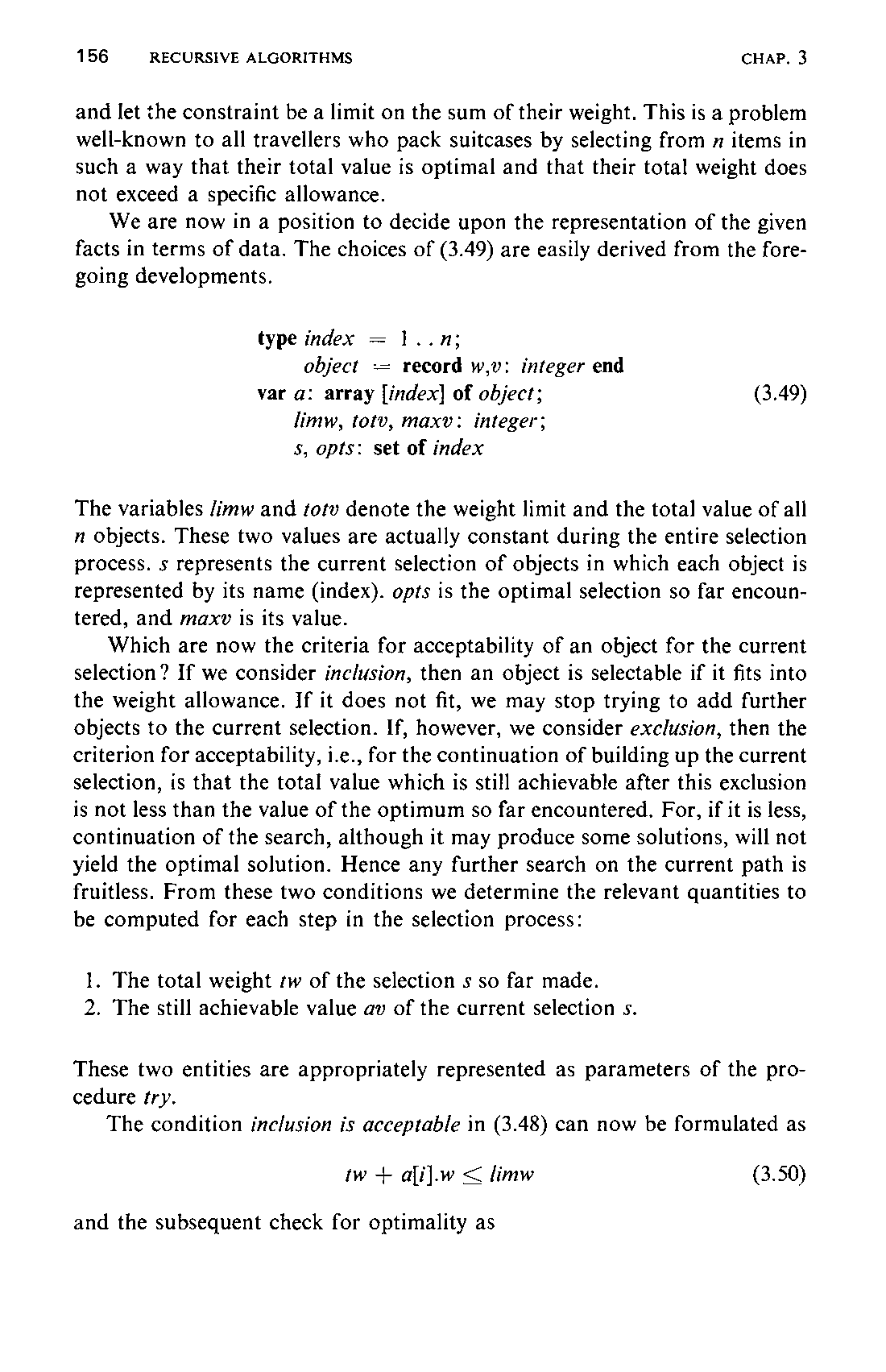
We are now in a position to decide upon the representation of the given facts in terms of data. The choices of (3.49) are easily derived from the foregoing developments.

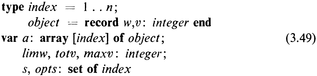
The variables /imw and totv denote the weight limit and the total value of all n objects. These two values are actually constant during the entire selection process. s represents the current selection of objects in which each object is represented by its name (index). opts is the optimal selection so far encountered, and maxv is its value.

Which are now the criteria for acceptability of an object for the current selection? If we consider inclusion, then an object is selectable if it fits into the weight allowance. If it does not fit, we may stop trying to add further objects to the current selection. If, however, we consider exclusion, then the criterion for acceptability, i.e., for the continuation of building up the current selection, is that the total value which is still achievable after this exclusion is not less than the value of the optimum so far encountered. For, if it is less, continuation of the search, although it may produce some solutions, will not yield the optimal solution. Hence any further search on the current path is fruitless. From these two conditions we determine the relevant quantities to be computed for each step in the selection process:

1. The total weight tw of the selection s so far made.

2. The still achievable value av of the current selection s.

These two entities are appropriately represented as parameters of the procedure try.

The condition inclusion is acceptable in (3.48) can now be formulated as

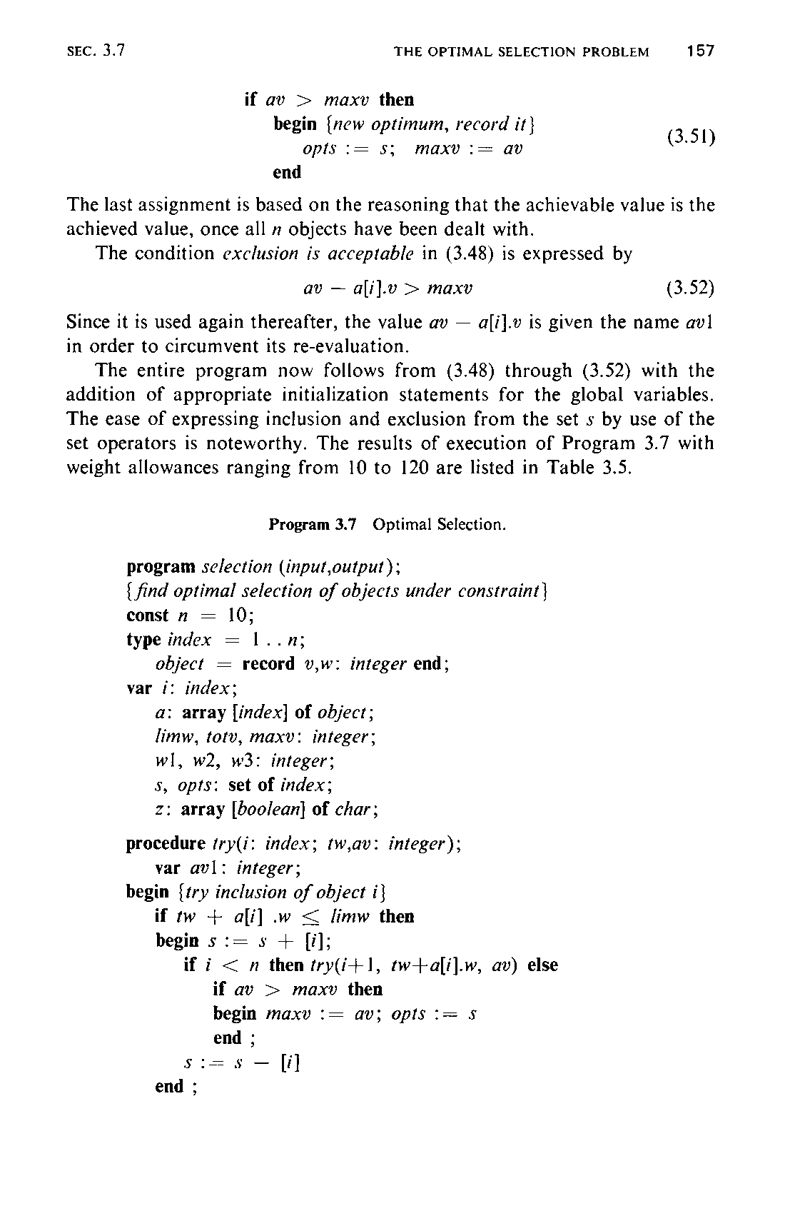
The last assignment is based on the reasoning that the achievable value is the achieved value, once all m objects have been dealt with.

Since it is used again thereafter, the value av — a[i].v is given the name avl in order to circumvent its re-evaluation.

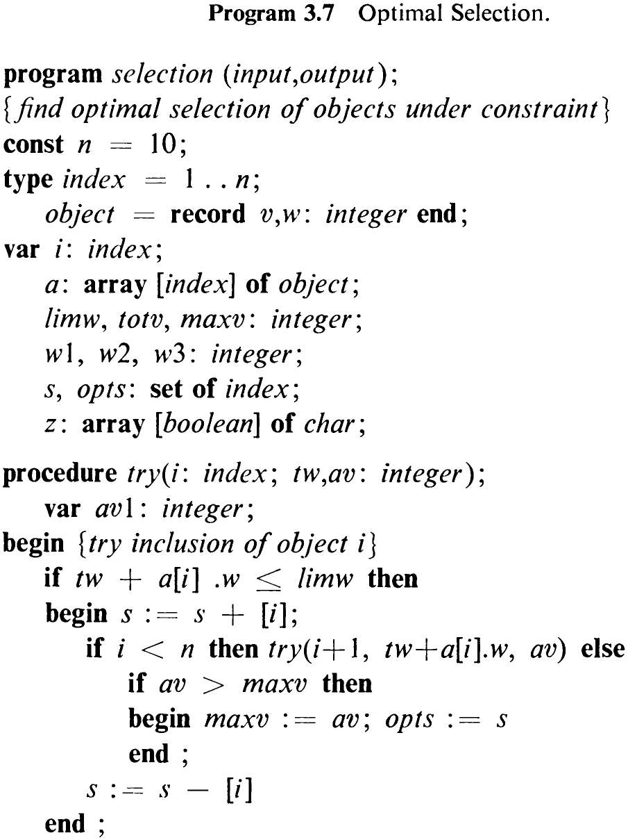
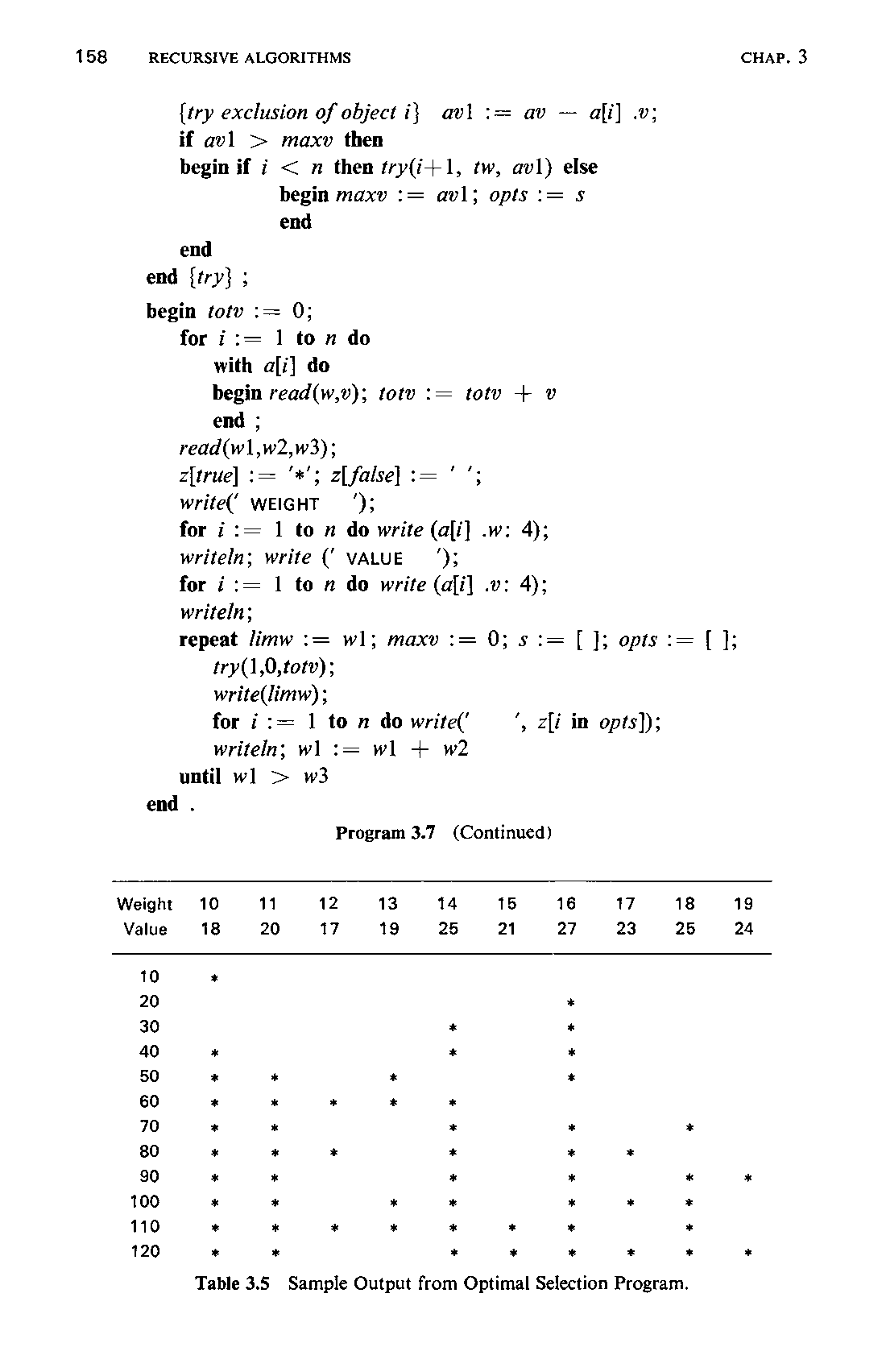
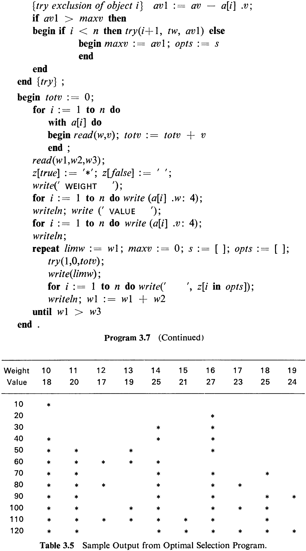
The entire program now follows from (3.48) through (3.52) with the addition of appropriate initialization statements for the global variables. The ease of expressing inclusion and exclusion from the set s by use of the set operators is noteworthy. The results of execution of Program 3.7 with weight allowances ranging from 10 to 120 are listed in Table 3.5.

This backtracking scheme with a limitation factor curtailing the growth of the potential search tree, is also known as branch and bound algorithm.