Sorting Sequential Files

2.3.1 Straight Merging

Unfortunately, the sorting algorithms presented in the preceding chapter are inapplicable if the amount of data to be sorted does not fit into a computer’s main store, but if it is, for instance, represented on a peripheral and sequential storage device such as a tape. In this case we describe the data as a (sequential) file whose characteristic is that at each moment one and only one component is directly accessible. This is a severe restriction compared to the possibilities offered by the array structure, and therefore different sorting techniques have to be used. The most important one is sorting by merging. Merging (or collating) means combining two (or more) ordered sequences into a single, ordered sequence by repeated selection among the currently accessible components. Merging is a much simpler operation than sorting, and it is used as an auxiliary operation in the more complex process of sequential sorting. One way of sorting on the basis of merging, called straight merging, is the following:

1. Split the sequence a into two halves, called b and c.

2. Merge b and c by combining single items into ordered pairs.

3. Call the merged sequence a, and repeat steps 1 and 2, this time merging ordered pairs into ordered quadruples.

4. Repeat the previous steps, merging quadruples into octets, and continue doing this, each time doubling the lengths of the merged subsequences, until the entire sequence is ordered.

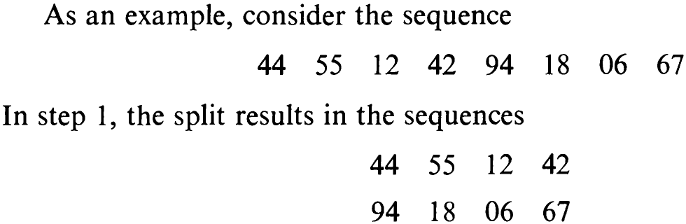
The merging of single components (which are ordered sequences of length 1), into ordered pairs yields

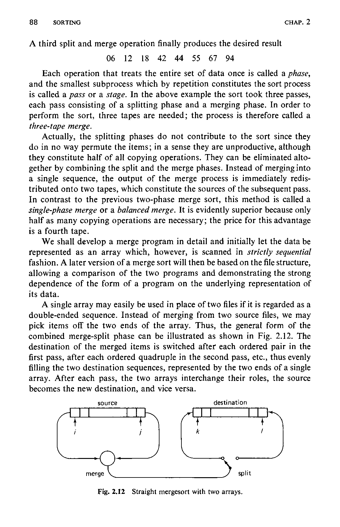
Each operation that treats the entire set of data once is called a phase, and the smallest subprocess which by repetition constitutes the sort process is called a pass or a stage. In the above example the sort took three passes, each pass consisting of a splitting phase and a merging phase. In order to perform the sort, three tapes are needed; the process is therefore called a three-tape merge.

Actually, the splitting phases do not contribute to the sort since they do in no way permute the items; in a sense they are unproductive, although they constitute half of all copying operations. They can be eliminated altogether by combining the split and the merge phases. Instead of merging into a single sequence, the output of the merge process is immediately redistributed onto two tapes, which constitute the sources of the subsequent pass. In contrast to the previous two-phase merge sort, this method is called a single-phase merge or a balanced merge. It is evidently superior because only half as many copying operations are necessary; the price for this advantage is a fourth tape.

We shall develop a merge program in detail and initially let the data be represented as an array which, however, is scanned in strictly sequential fashion. A later version of a merge sort will then be based on the file structure, allowing a comparison of the two programs and demonstrating the strong dependence of the form of a program on the underlying representation of its data.

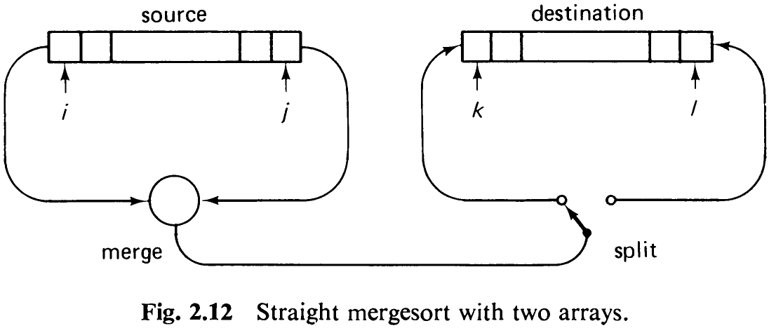
A single array may easily be used in place of two files if it is regarded as a double-ended sequence. Instead of merging from two source files, we may pick items off the two ends of the array. Thus, the general form of the combined merge-split phase can be illustrated as shown in Fig. 2.12. The destination of the merged items is switched after each ordered pair in the first pass, after each ordered quadruple in the second pass, etc., thus evenly filling the two destination sequences, represented by the two ends of a single array. After each pass, the two arrays interchange their roles, the source becomes the new destination, and vice versa.

A further simplification of the program can be achieved by joining the two conceptually distinct arrays into a single array of doubled size. Thus, the data will be represented by

and we let the indices i and j denote the two source items, whereas k and / designate the two destinations (see Fig. 2.12). The initial data are, of course, the items a, ...a,. Clearly, a Boolean variable up is needed to denote the direction of the data flow; up = true shall mean that in the current pass components a,...a, will be moved “up” to the variables a,,,...a),5 whereas up = false will indicate that a,,,...@,, Will be transferred “down” into a,...a,. The value of up strictly alternates between consecutive passes. And, finally, a variable p is introduced to denote the length of the subsequences to be merged. Its value is initially 1, and it is doubled before each successive pass. To simplify matters somewhat, we shall assume that nis always a power of 2. Thus, the first version of the straight merge program assumes the following form:

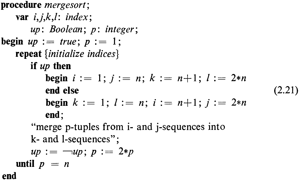
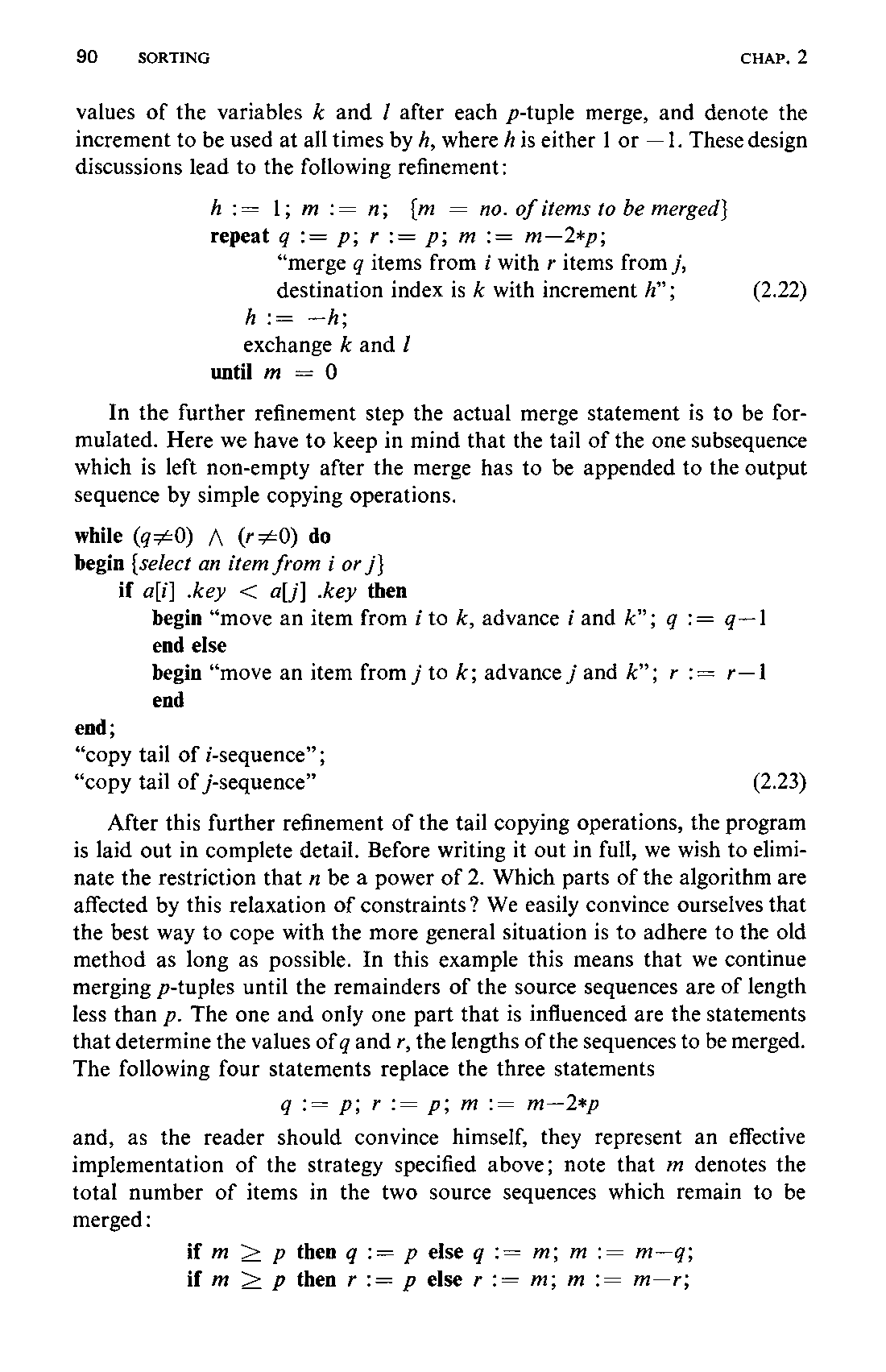
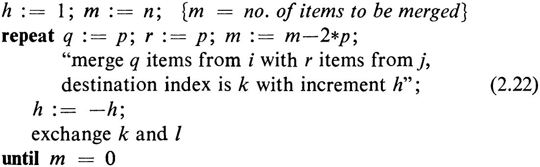
In the next development step we refine the statement expressed (within quotes) in natural language. Evidently, this merge pass involving n items is itself a sequence of merges of subsequences, i.e., of p-tuples. Between every such partial merge the destination is switched from the lower to the upper end of the destination array, or vice versa, to guarantee equal distribution onto both destinations. If the destination of the merged items is the lower end of the destination array, then the destination index is k, and k is incremented by 1 after each move of an item. If they are to be moved to the upper end of the destination array, the destination index is /, and / is to be decremented by | after each move. In order to simplify the actual merge statement, we choose the destination to be designated by k at all times, switching the90 values of the variables k and / after each p-tuple merge, and denote the increment to be used at all times by 4, where / is either 1 or —1. These design discussions lead to the following refinement:

In the further refinement step the actual merge statement is to be formulated. Here we have to keep in mind that the tail of the one subsequence which is left non-empty after the merge has to be appended to the output sequence by simple copying operations.

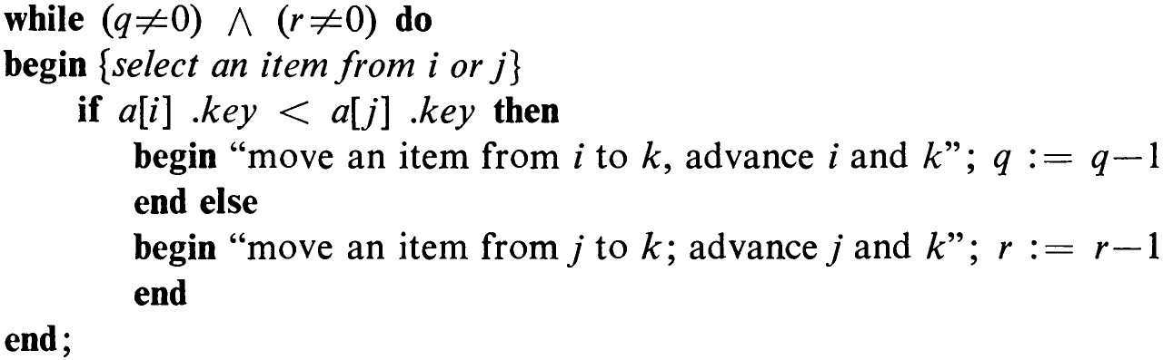
“copy tail of i-sequence”;

“copy tail of j-sequence” (2.23)

After this further refinement of the tail copying operations, the program is laid out in complete detail. Before writing it out in full, we wish to eliminate the restriction that n be a power of 2. Which parts of the algorithm are affected by this relaxation of constraints? We easily convince ourselves that the best way to cope with the more general situation is to adhere to the old method as long as possible. In this example this means that we continue merging p-tuples until the remainders of the source sequences are of length less than p. The one and only one part that is influenced are the statements that determine the values of q and r, the lengths of the sequences to be merged. The following four statements replace the three statements

and, as the reader should convince himself, they represent an effective implementation of the strategy specified above; note that m denotes the total number of items in the two source sequences which remain to be merged:

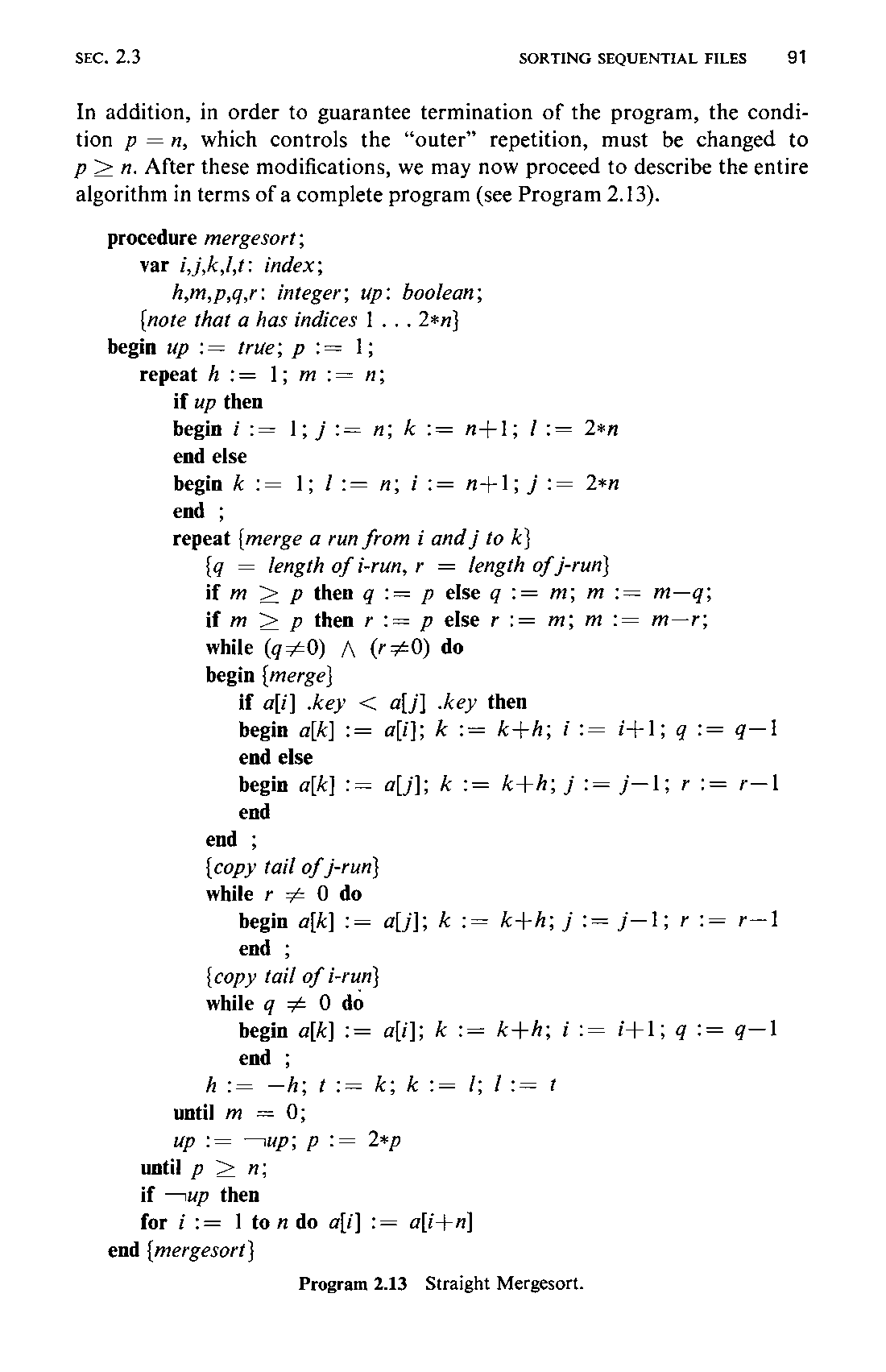
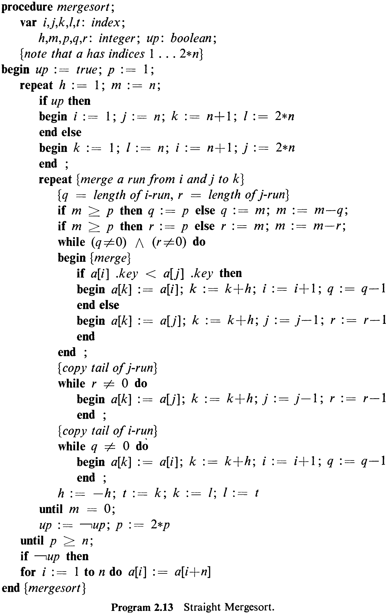
In addition, in order to guarantee termination of the program, the condition p =n, which controls the “outer” repetition, must be changed to p > n. After these modifications, we may now proceed to describe the entire algorithm in terms of a complete program (see Program 2.13).

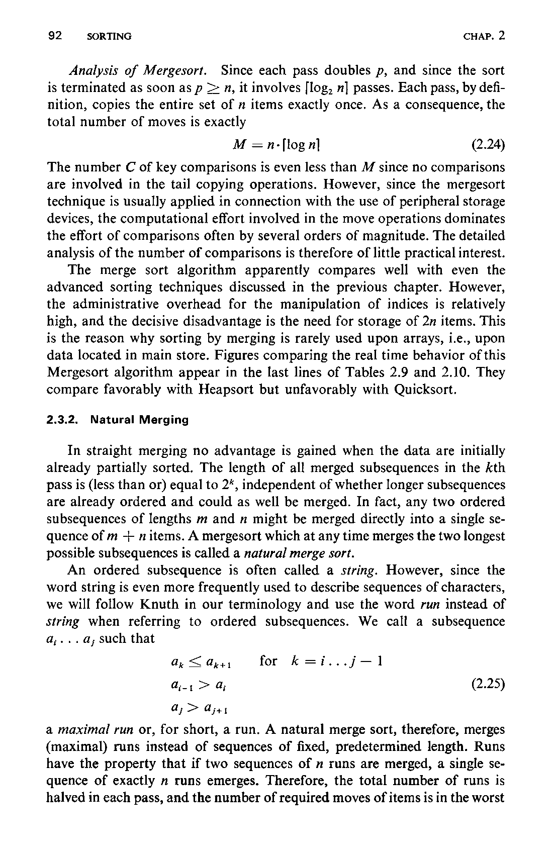
Analysis of Mergesort. Since each pass doubles p, and since the sort is terminated as soon as p > 4, it involves [log, n] passes. Each pass, by definition, copies the entire set of n items exactly once. As a consequence, the total number of moves is exactly

The number C of key comparisons is even less than M since no comparisons are involved in the tail copying operations. However, since the mergesort technique is usually applied in connection with the use of peripheral storage devices, the computational effort involved in the move operations dominates the effort of comparisons often by several orders of magnitude. The detailed analysis of the number of comparisons is therefore of little practical interest.

The merge sort algorithm apparently compares well with even the advanced sorting techniques discussed in the previous chapter. However, the administrative overhead for the manipulation of indices is relatively high, and the decisive disadvantage is the need for storage of 2n items. This is the reason why sorting by merging is rarely used upon arrays, i.e., upon data located in main store. Figures comparing the real time behavior of this Mergesort algorithm appear in the last lines of Tables 2.9 and 2.10. They compare favorably with Heapsort but unfavorably with Quicksort.

2.3.2 Natural Merging

In straight merging no advantage is gained when the data are initially already partially sorted. The length of all merged subsequences in the kth pass is (less than or) equal to 2*, independent of whether longer subsequences are already ordered and could as well be merged. In fact, any two ordered subsequences of lengths m and n might be merged directly into a single sequence of m + nitems. A mergesort which at any time merges the two longest possible subsequences is called a natural merge sort.

An ordered subsequence is often called a string. However, since the word string is even more frequently used to describe sequences of characters, we will follow Knuth in our terminology and use the word run instead of string when referring to ordered subsequences. We call a subsequence a;...a, such that

a maximal run or, for short, a run. A natural merge sort, therefore, merges (maximal) runs instead of sequences of fixed, predetermined length. Runs have the property that if two sequences of n runs are merged, a single sequence of exactly m runs emerges. Therefore, the total number of runs is halved in each pass, and the number of required moves of items is in the worst93 case n-[log, n], but in the average case it is even less. The expected number of comparisons, however, is much larger because in addition to the comparisons necessary for the selection of items, further comparisons are needed between consecutive items of each file in order to determine the end of each

run.

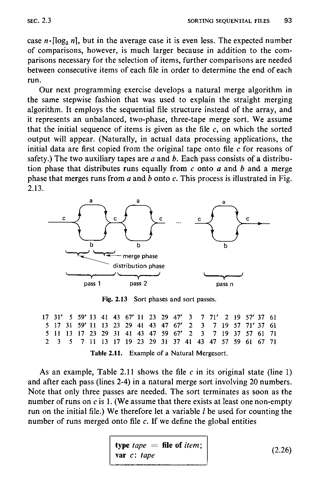
Our next programming exercise develops a natural merge algorithm in the same stepwise fashion that was used to explain the straight merging algorithm. It employs the sequential file structure instead of the array, and it represents an unbalanced, two-phase, three-tape merge sort. We assume that the initial sequence of items is given as the file c, on which the sorted output will appear. (Naturally, in actual data processing applications, the initial data are first copied from the original tape onto file c for reasons of safety.) The two auxiliary tapes are a and b. Each pass consists of a distribution phase that distributes runs equally from c onto a and b and a merge phase that merges runs from a and b onto c. This process is illustrated in Fig.

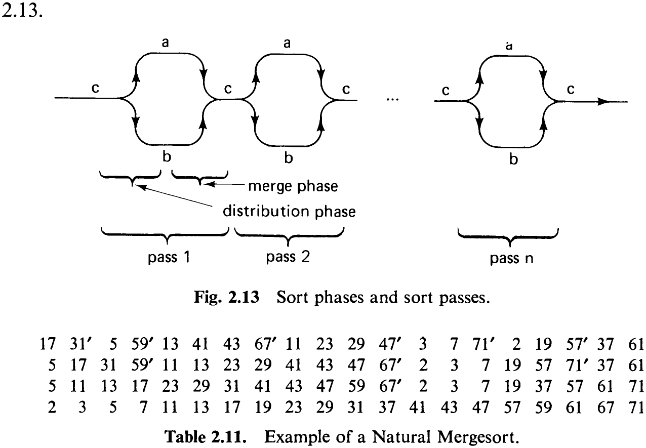
As an example, Table 2.11 shows the file c in its original state (line 1) and after each pass (lines 2-4) in a natural merge sort involving 20 numbers. Note that only three passes are needed. The sort terminates as soon as the number of runs on c is 1. (We assume that there exists at least one non-empty run on the initial file.) We therefore let a variable / be used for counting the number of runs merged onto file c. If we define the global entities

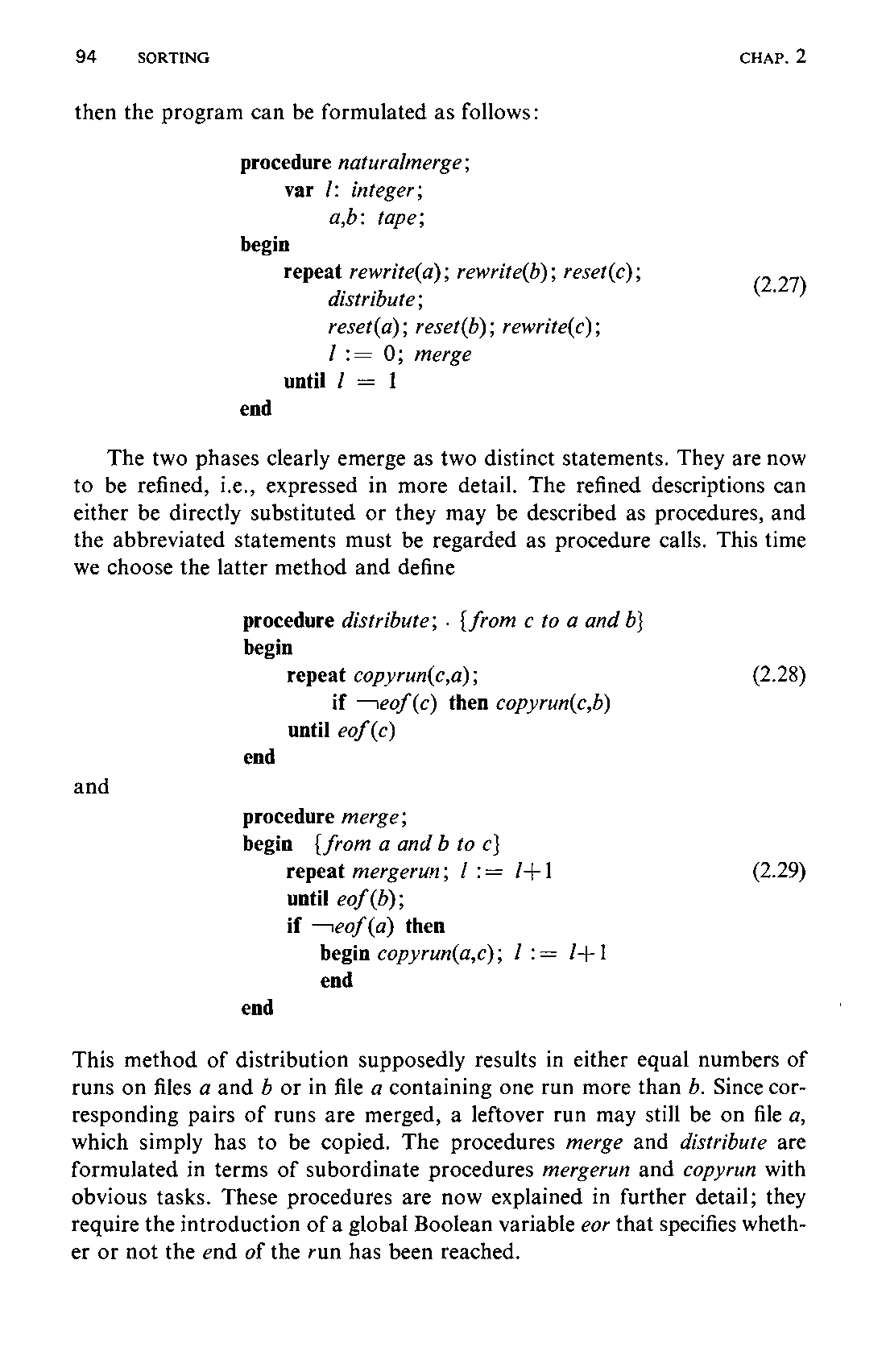
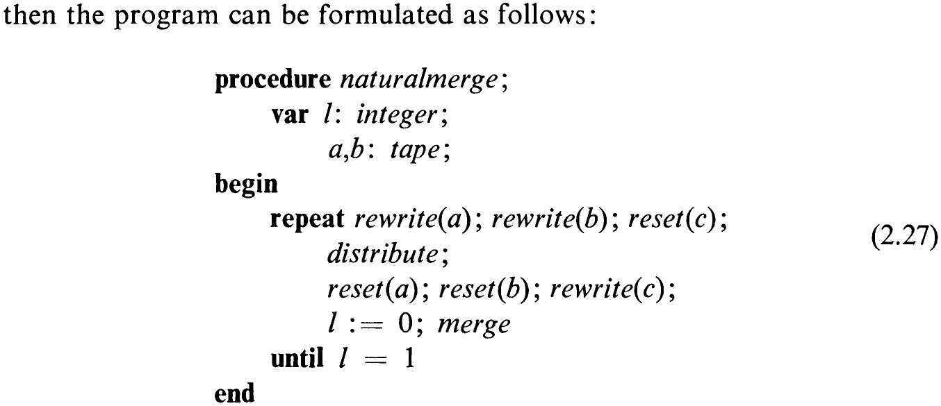
The two phases clearly emerge as two distinct statements. They are now to be refined, i.e., expressed in more detail. The refined descriptions can either be directly substituted or they may be described as procedures, and the abbreviated statements must be regarded as procedure calls. This time we choose the latter method and define

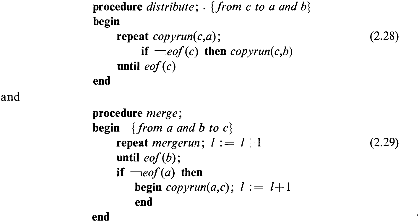
This method of distribution supposedly results in either equal numbers of runs on files a and 5 or in file a containing one run more than B. Since corresponding pairs of runs are merged, a leftover run may still be on file a, which simply has to be copied. The procedures merge and distribute are formulated in terms of subordinate procedures mergerun and copyrun with obvious tasks. These procedures are now explained in further detail; they require the introduction of a global Boolean variable eor that specifies whether or not the end of the run has been reached.

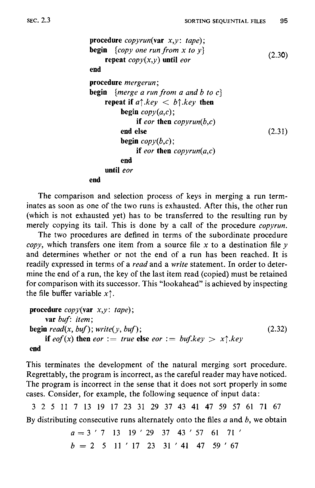
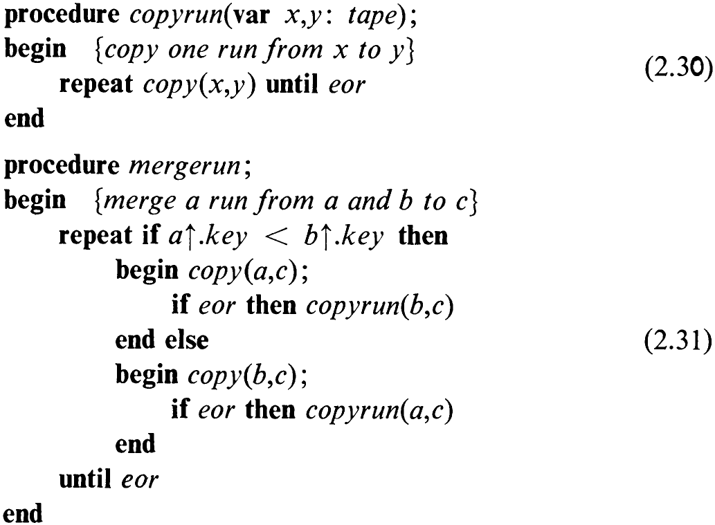
The comparison and selection process of keys in merging a run terminates as soon as one of the two runs is exhausted. After this, the other run (which is not exhausted yet) has to be transferred to the resulting run by merely copying its tail. This is done by a call of the procedure copyrun.

The two procedures are defined in terms of the subordinate procedure copy, which transfers one item from a source file x to a destination file y and determines whether or not the end of a run has been reached. It is readily expressed in terms of a read and a write statement. In order to determine the end of a run, the key of the last item read (copied) must be retained for comparison with its successor. This “lookahead” is achieved by inspecting the file buffer variable x7.

begin read(x, buf); write(y, buf); (2.32)

This terminates the development of the natural merging sort procedure. Regrettably, the program is incorrect, as the careful reader may have noticed. The program is incorrect in the sense that it does not sort properly in some cases. Consider, for example, the following sequence of input data:

By distributing consecutive runs alternately onto the files a and b, we obtain

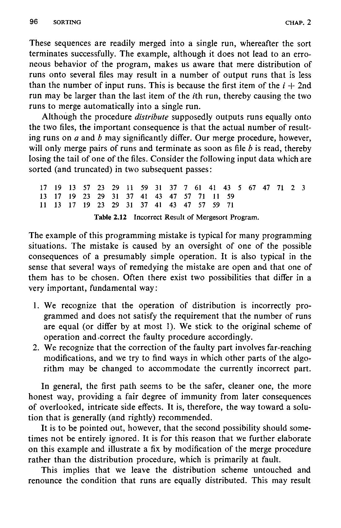
These sequences are readily merged into a single run, whereafter the sort terminates successfully. The example, although it does not lead to an erroneous behavior of the program, makes us aware that mere distribution of runs onto several files may result in a number of output runs that is less than the number of input runs. This is because the first item of the i + 2nd run may be larger than the last item of the ith run, thereby causing the two runs to merge automatically into a single run.

Although the procedure distribute supposedly outputs runs equally onto the two files, the important consequence is that the actual number of resulting runs on a and b may significantly differ. Our merge procedure, however, will only merge pairs of runs and terminate as soon as file b is read, thereby losing the tail of one of the files. Consider the following input data which are sorted (and truncated) in two subsequent passes:

The example of this programming mistake is typical for many programming situations. The mistake is caused by an oversight of one of the possible consequences of a presumably simple operation. It is also typical in the sense that several ways of remedying the mistake are open and that one of them has to be chosen. Often there exist two possibilities that differ in a very important, fundamental way:

1. We recognize that the operation of distribution is incorrectly programmed and does not satisfy the requirement that the number of runs are equal (or differ by at most 1). We stick to the original scheme of operation and.correct the faulty procedure accordingly.

2. We recognize that the correction of the faulty part involves far-reaching modifications, and we try to find ways in which other parts of the algorithm may be changed to accommodate the currently incorrect part.

In general, the first path seems to be the safer, cleaner one, the more honest way, providing a fair degree of immunity from later consequences of overlooked, intricate side effects. It is, therefore, the way toward a solution that is generally (and rightly) recommended.

It is to be pointed out, however, that the second possibility should sometimes not be entirely ignored. It is for this reason that we further elaborate on this example and illustrate a fix by modification of the merge procedure rather than the distribution procedure, which is primarily at fault.

This implies that we leave the distribution scheme untouched and renounce the condition that runs are equally distributed. This may result97 in a less than optimal performance. However, the worst-case performance remains unchanged, and, moreover, the case of highly unequal distribution is statistically very unlikely. Efficiency considerations are therefore no serious argument against this solution.

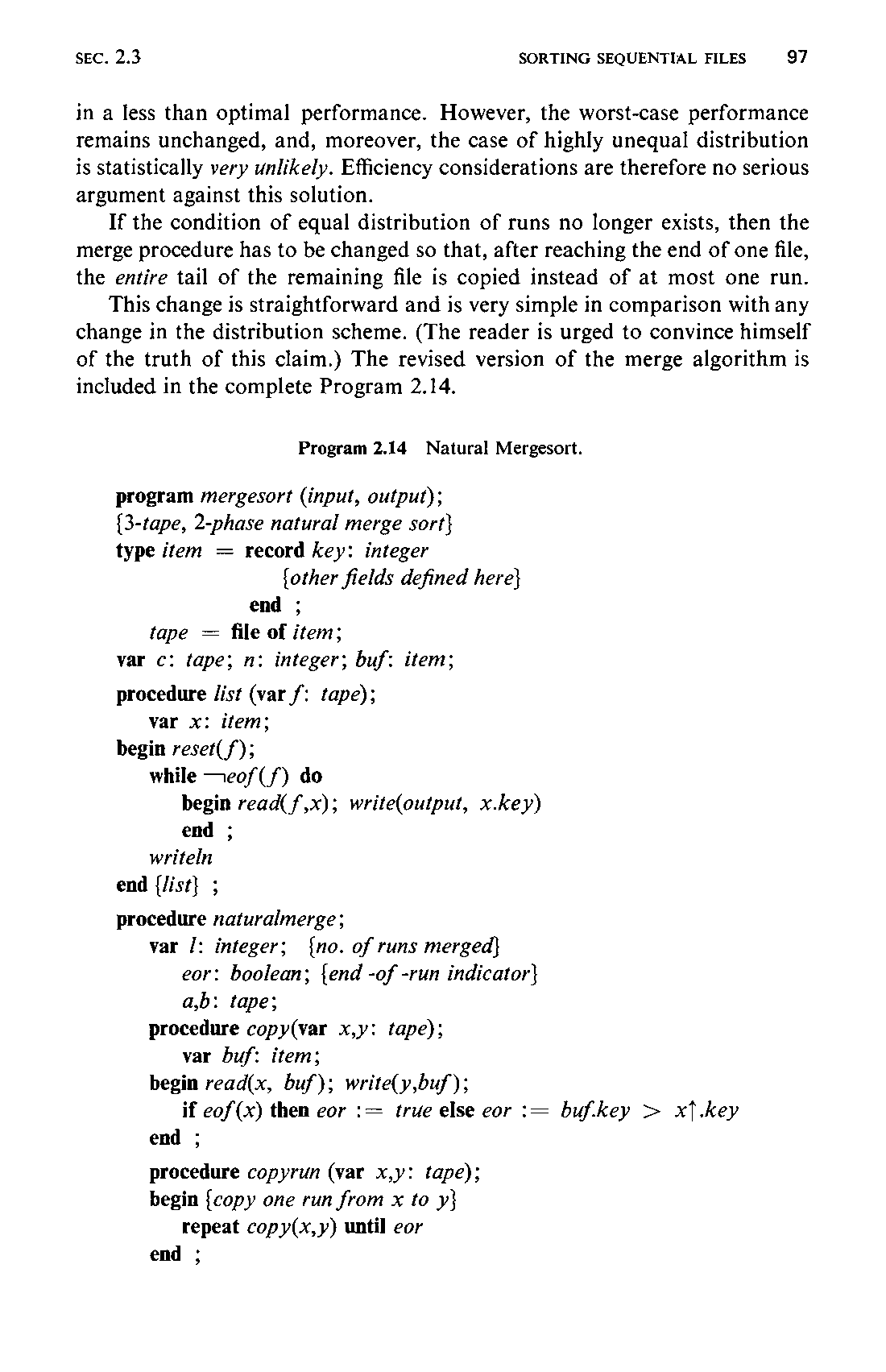
If the condition of equal distribution of runs no longer exists, then the merge procedure has to be changed so that, after reaching the end of one file, the entire tail of the remaining file is copied instead of at most one run.

This change is straightforward and is very simple in comparison with any change in the distribution scheme. (The reader is urged to convince himself of the truth of this claim.) The revised version of the merge algorithm is included in the complete Program 2.14.

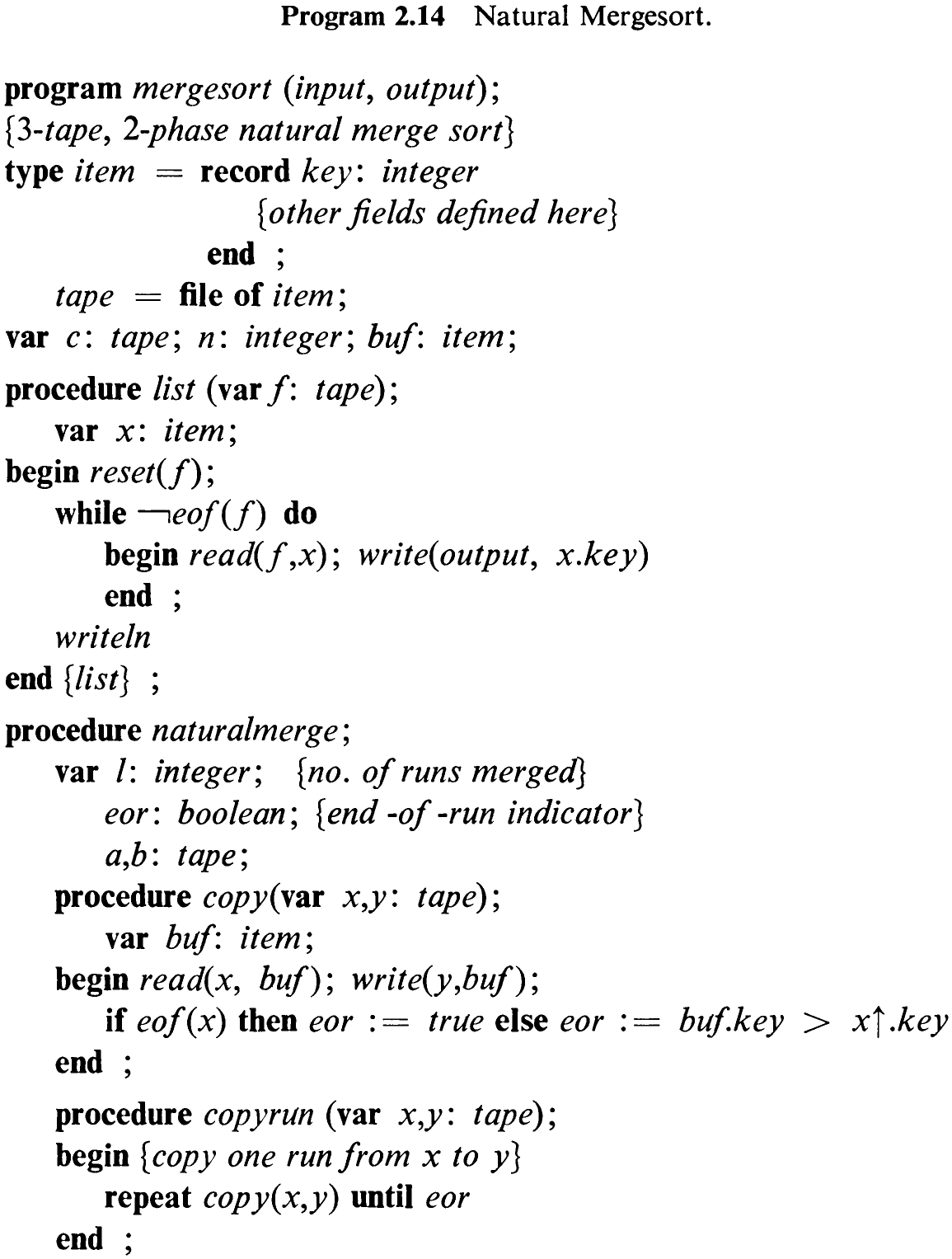
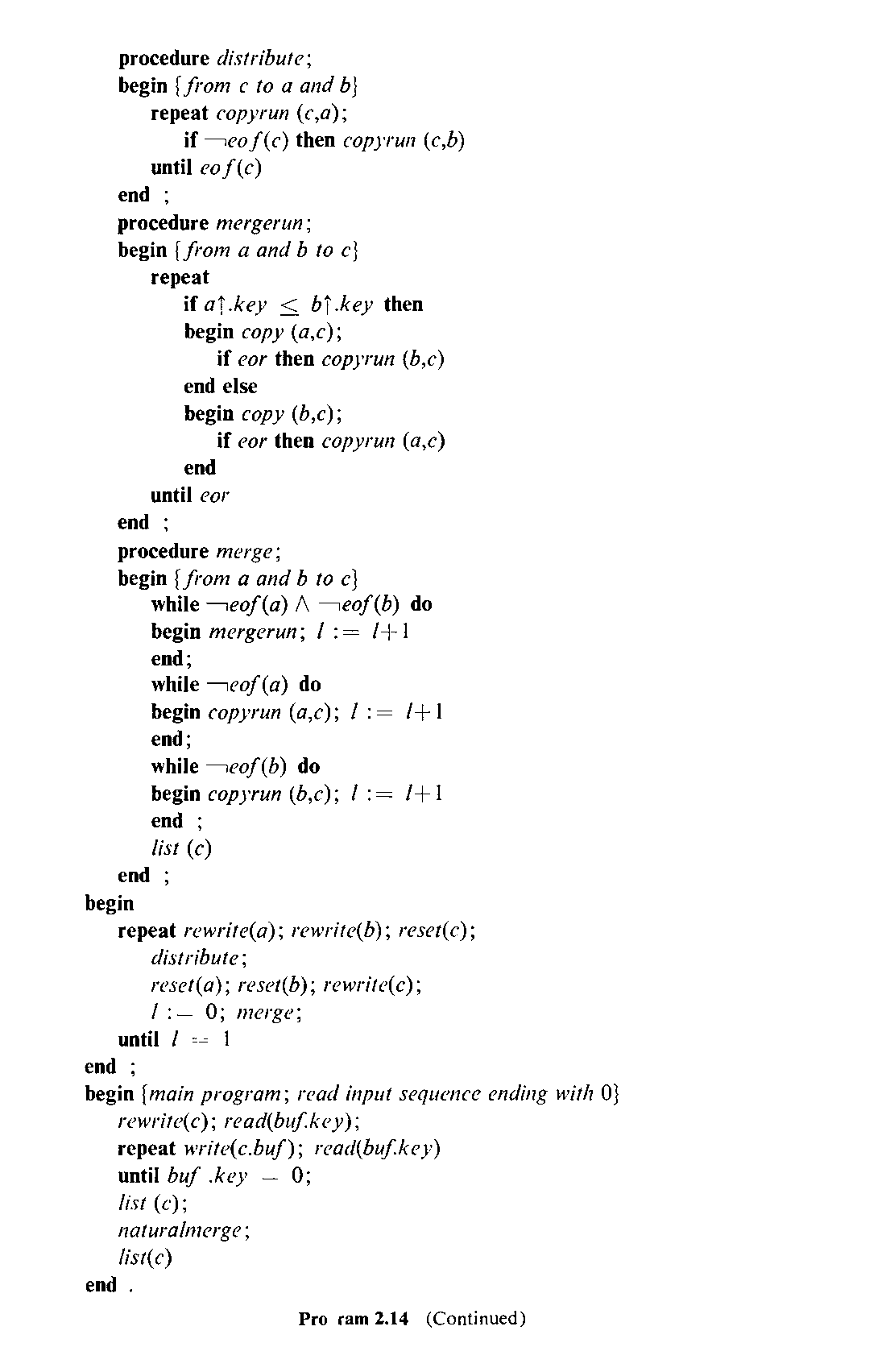
   procedure distribute;
   begin {from c to a and b}
      repeat copyrun (c,a);
         if ¬eof(c) then copyrun (c,b)
      until eof(c)
   end ;
   procedure mergerun;
   begin {from a and b to c}
      repeat
         if a↑.key ≤ b↑.key then
         begin copy (a,c);
            if eor then copyrun (b,c)
         end else
         begin copy (b,c);
            if eor then copyrun (a,c)
         end
      until eor
   end ;
   procedure merge;
   begin {from a and b to c}
      while ¬eof(a) ∧ ¬eof(b) do
      begin mergerun; l := l+1
      end;
      while ¬eof(a) do
      begin copyrun (a,c); l := l+1
      end;
      while ¬eof(b) do
      begin copyrun (b,c); l := l+1
      end ;
      list (c)
   end ;
begin
   repeat rewrite(a); rewrite(b); reset(c);
      distribute;
      reset(a); reset(b); rewrite(c);
      l := 0; merge;
   until l = 1
end ;
begin {main program; read input sequence ending with 0}
   rewrite(c); read(buf.key);
   repeat write(c.buf); read(buf.key)
   until buf.key = 0;
   list (c);
   naturalmerge;
   list(c)
end .

2.3.3 Balanced Multiway Merging

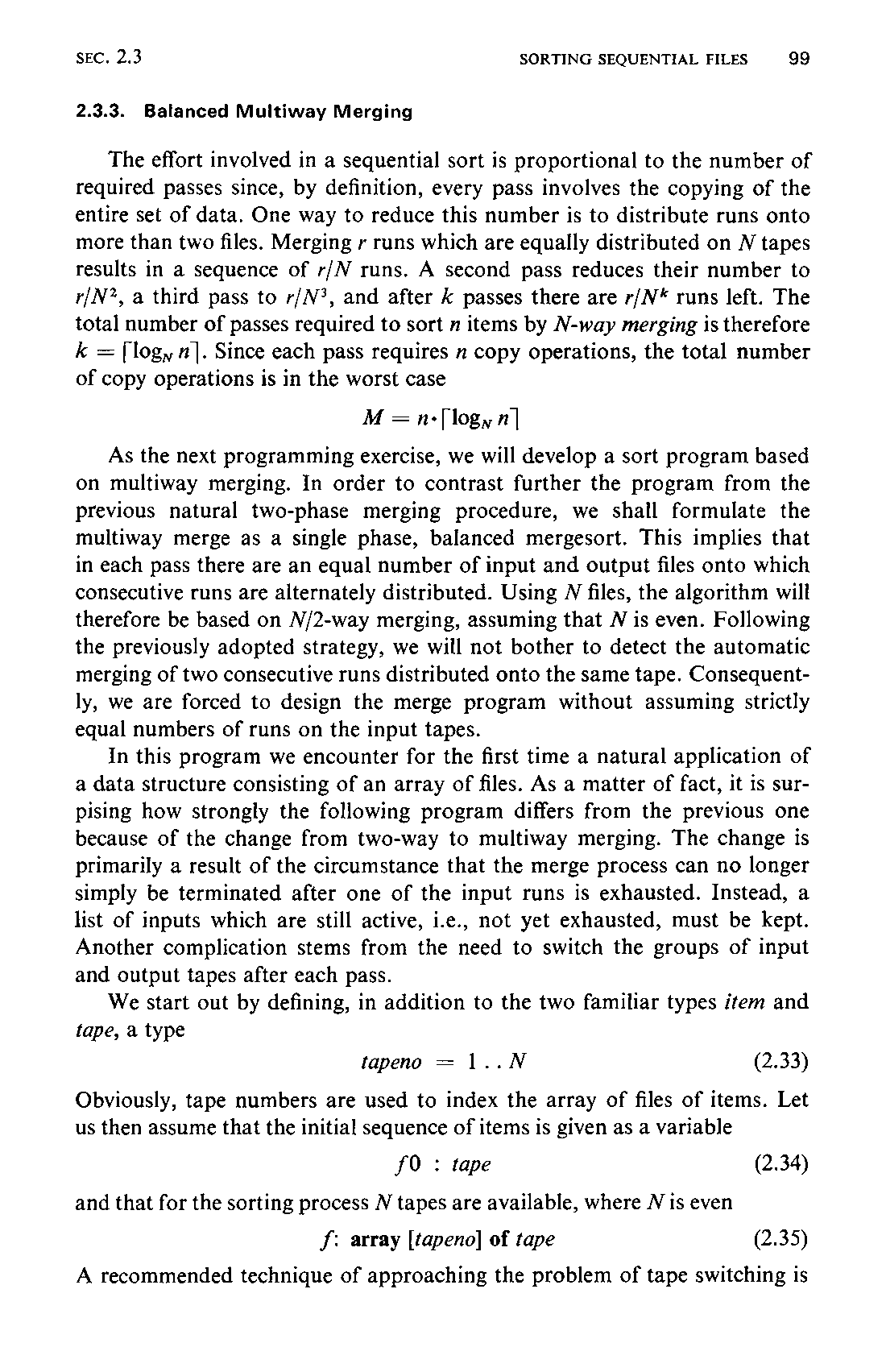
The effort involved in a sequential sort is proportional to the number of required passes since, by definition, every pass involves the copying of the entire set of data. One way to reduce this number is to distribute runs onto more than two files. Merging $r$ runs which are equally distributed on $N$ tapes results in a sequence of $r/N$ runs. A second pass reduces their number to $r/N^2$, a third pass to $r/N^3$, and after $k$ passes there are $r/N^k$ runs left. The total number of passes required to sort $n$ items by $N$-way merging is therefore $k = \lceil \log_N n \rceil$. Since each pass requires $n$ copy operations, the total number of copy operations is in the worst case

As the next programming exercise, we will develop a sort program based on multiway merging. In order to contrast further the program from the previous natural two-phase merging procedure, we shall formulate the multiway merge as a single phase, balanced mergesort. This implies that in each pass there are an equal number of input and output files onto which consecutive runs are alternately distributed. Using $N$ files, the algorithm will therefore be based on $N/2$-way merging, assuming that $N$ is even. Following the previously adopted strategy, we will not bother to detect the automatic merging of two consecutive runs distributed onto the same tape. Consequently, we are forced to design the merge program without assuming strictly equal numbers of runs on the input tapes.

In this program we encounter for the first time a natural application of a data structure consisting of an array of files. As a matter of fact, it is surpising how strongly the following program differs from the previous one because of the change from two-way to multiway merging. The change is primarily a result of the circumstance that the merge process can no longer simply be terminated after one of the input runs is exhausted. Instead, a list of inputs which are still active, i.e., not yet exhausted, must be kept. Another complication stems from the need to switch the groups of input and output tapes after each pass.

We start out by defining, in addition to the two familiar types item and tape, a type

tapeno = 1 .. N

Obviously, tape numbers are used to index the array of files of items. Let us then assume that the initial sequence of items is given as a variable

f0 : tape

and that for the sorting process $N$ tapes are available, where $N$ is even

f: array [tapeno] of tape

A recommended technique of approaching the problem of tape switching is100 to introduce a tape index map. Instead of directly addressing a tape by its index $i$, it is addressed via a map $t$, i.e., instead of each

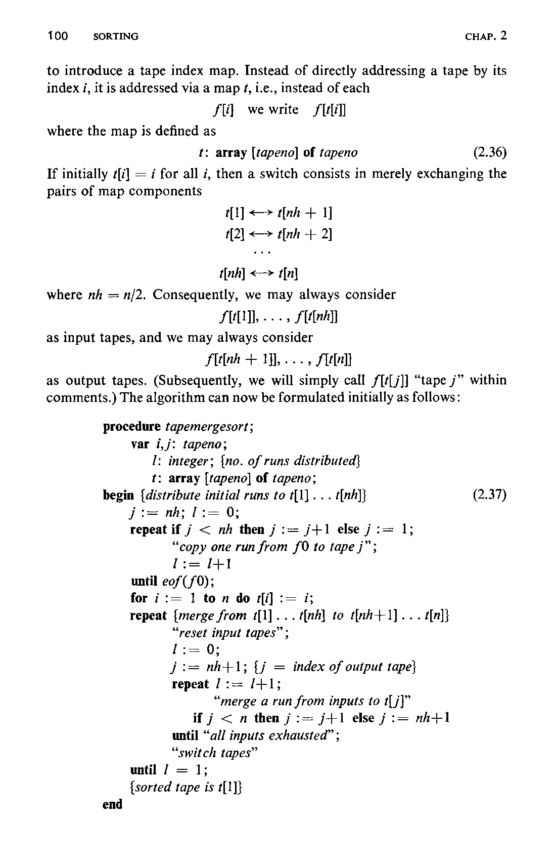
where the map is defined as

t: array [tapeno] of tapeno

If initially $t[i] = i$ for all $i$, then a switch consists in merely exchanging the pairs of map components

where $nh = n/2$. Consequently, we may always consider

as input tapes, and we may always consider

as output tapes. (Subsequently, we will simply call f[t[j]] “tape $j$” within comments.) The algorithm can now be formulated initially as follows:

procedure tapemergesort;
    var i,j: tapeno;
        l: integer; {no. of runs distributed}
        t: array [tapeno] of tapeno;
begin {distribute initial runs to t[1] ... t[nh]}
    j := nh; l := 0;
    repeat if j < nh then j := j+1 else j := 1;
           “copy one run from f0 to tape j”;
           l := l+1
    until eof(f0);
    for i := 1 to n do t[i] := i;
    repeat {merge from t[1] ... t[nh] to t[nh+1] ... t[n]}
           “reset input tapes”;
           l := 0;
           j := nh+1; {j = index of output tape}
           repeat l := l+1;
                  “merge a run from inputs to t[j]”
              if j < n then j := j+1 else j := nh+1
           until “all inputs exhausted”;
           “switch tapes”
    until l = 1;
    {sorted tape is t[1]}
end

101 First, we refine the copy operation used in the initial distribution of runs; we again introduce an auxiliary variable to buffer the last item read:

buf: item

and replace “copy one run from f0 to tape $j$” by the statement

repeat read(f0, buf);
    write(f[j], buf)
until (buf.key > f0↑.key) ∨ eof(f0)

Copying a run terminates when either the first item of the next run is encountered (buf.key > f0↑.key) or when the end of the entire input file is reached (eof(f0)).

In the actual sort algorithm there remain the statements

1. Reset input tapes
2. Merge a run from inputs to $t[j]$
3. Switch tapes

and the predicate

4. All inputs exhausted

to be specified in more detail. First, we must accurately identify the current input files. Notably, the number of “active” input files may be less than $n/2$. In fact, there can be at most as many sources as there are runs; the sort terminates as soon as there is one single file left. This leaves open the possibility that at the initiation of the last sort pass there are fewer than nh runs. We therefore introduce a variable, say k1, to denote the actual number of input files used. We incorporate the initialization of k1 in the statement “reset input tapes” as follows:

if l < nh then k1 := l else k1 := nh;
for i := 1 to k1 do reset(f[t[i]]);

Naturally, statement (2) is to decrement k1 whenever an input source ceases. Hence, predicate (4) may easily be expressed by the relation

Statement (2) is more difficult to refine; it consists of the repeated selection of the least key among the available sources and its subsequent transport to the destination, i.e., the current output tape. The process is complicated again by the necessity of determining the end of each run. The end of a run may be reached because (1) the subsequent key is less than the current key or (2) the end of the source file is reached. In the latter case the tape is eliminated by decrementing k1; in the former case the run is closed by excluding the file from further selection of items, but only until the creation of the current output run is completed. This makes it obvious that a second102 variable, say k2, is needed to denote the number of source tapes actually available for the selection of the next item. This value is initially set equal to k1 and is decremented whenever a run terminates because of condition (1).

Unfortunately, the introduction of k2 is not enough; knowledge of the number of tapes does not suffice. We need to know exactly which tapes are still in the game. An obvious solution is to use an array with Boolean components indicating the availability of the tapes. We choose, however, a different method which leads to a more efficient selection procedure which, after all, is the most frequently repeated part of the entire algorithm. Instead of using a Boolean array, a second tape map, say ta, is introduced. This map is used in place of $t$ such that ta[1] … ta[k2] are the indices of the tapes available. Thus statement (2) can be formulated as follows:

k2 := k1;
repeat “select the minimal key, let ta[mx] be its tape number”;
       read(f[ta[mx]], buf);
       write(f[t[j]], buf);
       if eof(f[ta[mx]]) then “eliminate tape” else
       if buf.key > f[ta[mx]]↑.key then “close run”
until k2 = 0

Since the number of tape units available in any computer installation is usually fairly small, the selection algorithm to be specified in further detail in the next refinement step may as well be a straightforward linear search. The statement “eliminate tape” implies a decrease of k1 as well as k2 and implies a re-assignment of indices in the map ta. The statement “close run” merely decrements k2 and re-arranges components of ta accordingly. The details are shown in Program 2.15, which is a last refinement of (2.37)

program balancedmerge (output);
{balanced n-way tape merge sort}
const n = 6; nh = 3;         {no. of tapes}
type item = record
               key: integer
            end ;
   tape = file of item;
   tapeno = 1 .. n;
var leng, rand: integer;     {used to generate file}
   eot: boolean;             {end of tape}
   buf: item;
   f0: tape; {f0 is the input tape with random numbers}
   f: array [1 .. n] of tape;
procedure list(var f: tape; n: tapeno);
   var z: integer;
begin writeln('TAPE', n:2); z := 0;
   while ¬eof(f) do
   begin read(f, buf); write(output, buf.key: 5); z := z+1;
      if z = 25 then
         begin writeln(output); z := 0;
         end
   end ;
   if z ≠ 0 then writeln (output); reset(f)
end {list} ;

procedure tapemergesort;
   var i,j,mx,tx: tapeno;
      k1,k2,l; integer;
      x, min: integer;
      t, ta: array [tapeno] of tapeno;
begin {distribute initial runs to t[1] ... t[nh]}
   for i := 1 to nh do rewrite(f[i]);
   j := nh; l := 0;
   repeat if j < nh then j := j+1 else j := 1;
      {copy one run from f0 to tape j}
      l := l+1;
      repeat read(f0, buf); write(f[j], buf)
      until (buf.key > f0↑.key) ∨ eof(f0)
   until eof(f0);
   for i := 1 to n do t[i] := i;
   repeat {merge from t[1] ... t[nh] to t[nh+1] ... t[n]}
      if l < nh then k1 := l else k1 := nh;
      {k1 = no. of input tapes in this phase}
      for i := 1 to k1 do
         begin reset(f[t[i]]); list(f[t[i]], t[i]); ta[i] := t[i]
         end ;
      l := 0;  {l = number of runs merged}
      j := nh+1;     {j = index of output tape}
      repeat {merge a run from t[1] ... t[k1] to t[j]}
         k2 := k1; l := l+1;  {k2 = no. of active input tapes}
         repeat {select minimal element}
            i := 1; mx := 1; min := f[ta[1]]↑.key;
            while i < k2 do
            begin i := i+1; x := f[ta[i]]↑.key;
                  if x < min then
                  begin min := x; mx := i
                  end
            end ;
            {ta[mx] has minimal element, move it to t[j]}
            read(f[ta[mx]], buf); eot := eof(f[ta[mx]]);
            write(f[t[j]], buf);
            if eot then
            begin rewrite(f[ta[mx]]); {eliminate tape}
               ta[mx] := ta[k2]; ta[k2] := ta[k1];
               k1 := k1-1; k2 := k2-1
            end else
            if buf.key > f[ta[mx]]↑.key then
            begin tx := ta[mx]; ta[mx] := ta[k2]; ta[k2] := tx;
               k2 := k2-1
            end
         until k2 = 0;
         if j < n then j := j+1 else j := nh+1
      until k1 = 0;
      for i := 1 to nh do
         begin tx := t[i]; t[i] := t[i+nh]; t[i+nh] := tx
         end
   until l = 1;
   reset(f[t[1]]); list(f[t[1]], t[1]);  {sorted output is on t[1]}
end {tapemergesort} ;

begin {generate random file f0}
   leng := 200; rand := 7789; rewrite(f0);
   repeat rand := (131071*rand) mod 2147483647;
      buf.key := rand div 2147484; write(f0, buf); leng := leng - 1
   until leng = 0;
   reset(f0); list(f0, 1);
   tapemergesort
end .

through (2.39). Note that tapes are rewound by the procedure rewrite as soon as their last run has been read. The statement “switch tapes” is elaborated according to explanations given earlier.

2.3.4 Polyphase Sort

We have now discussed the necessary techniques and have acquired the proper background to investigate and program yet another sorting algorithm whose performance is superior to the balanced sort. We have seen that balanced merging eliminates the pure copying operations necessary when the distribution and the merging operations are united into a single phase.105 The question arises whether or not the given tapes could still be better utilized. This is indeed the case; the key to this next improvement lies in abandoning the rigid notion of strict passes, i.e., to use the tapes in a more sophisticated way than by always having $N/2$ source tapes and as many destination tapes and exchanging source and destination tapes at the end of each distinct pass. Instead, the notion of a pass becomes diffuse. The method was invented by R. L. Gilstad [2-3] and christened Polyphase Sort.

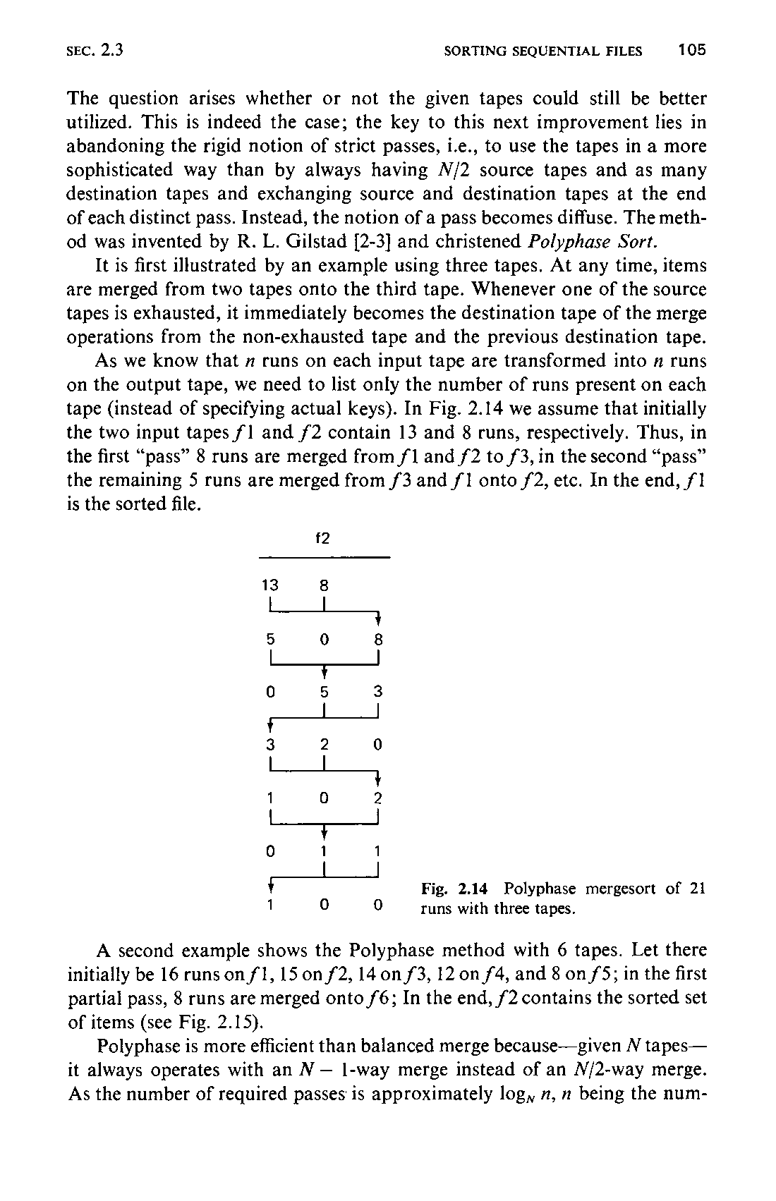
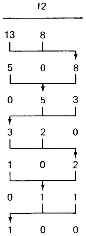
It is first illustrated by an example using three tapes. At any time, items are merged from two tapes onto the third tape. Whenever one of the source tapes is exhausted, it immediately becomes the destination tape of the merge operations from the non-exhausted tape and the previous destination tape.

As we know that $n$ runs on each input tape are transformed into $n$ runs on the output tape, we need to list only the number of runs present on each tape (instead of specifying actual keys). In Fig. 2.14 we assume that initially the two input tapes f1 and f2 contain 13 and 8 runs, respectively. Thus, in the first “pass” 8 runs are merged from f1 and f2 to f3, in the second “pass” the remaining 5 runs are merged from f3 and f1 onto f2, etc. In the end, f1 is the sorted file.

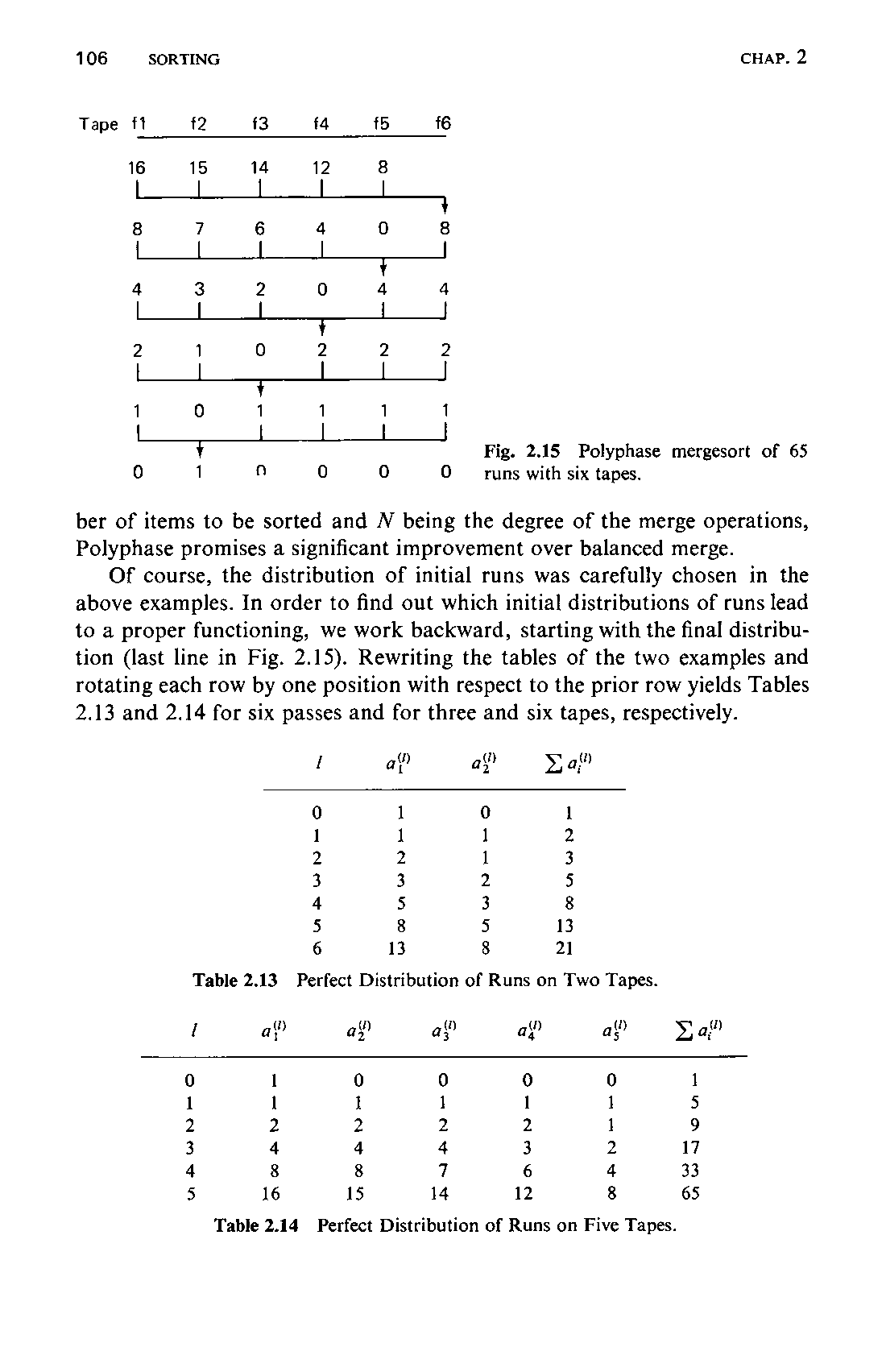
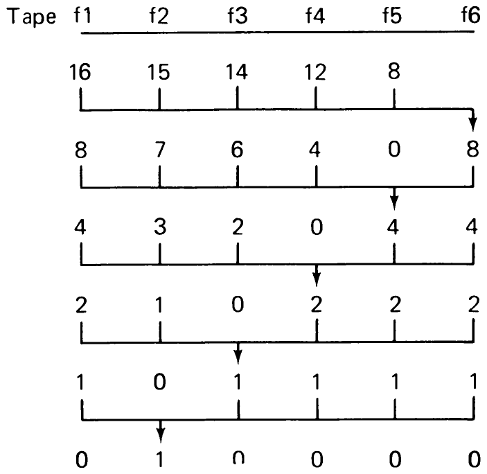
A second example shows the Polyphase method with 6 tapes. Let there initially be 16 runs on f1, 15 on f2, 14 on f3, 12 on f4, and 8 on f5; in the first partial pass, 8 runs are merged onto f6; In the end, f2 contains the sorted set of items (see Fig. 2.15).

Polyphase is more efficient than balanced merge because—given $N$ tapes—it always operates with an $N - 1$-way merge instead of an $N/2$-way merge. As the number of required passes is approximately $\log_N n$, $n$ being the number106 of items to be sorted and $N$ being the degree of the merge operations, Polyphase promises a significant improvement over balanced merge.

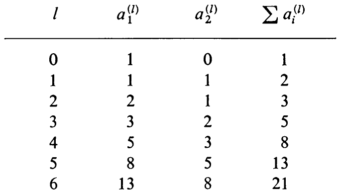
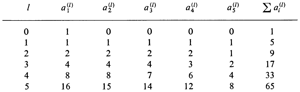
Of course, the distribution of initial runs was carefully chosen in the above examples. In order to find out which initial distributions of runs lead to a proper functioning, we work backward, starting with the final distribution (last line in Fig. 2.15). Rewriting the tables of the two examples and rotating each row by one position with respect to the prior row yields Tables 2.13 and 2.14 for six passes and for three and six tapes, respectively.

107 From Table 2.13 we can deduce the relations

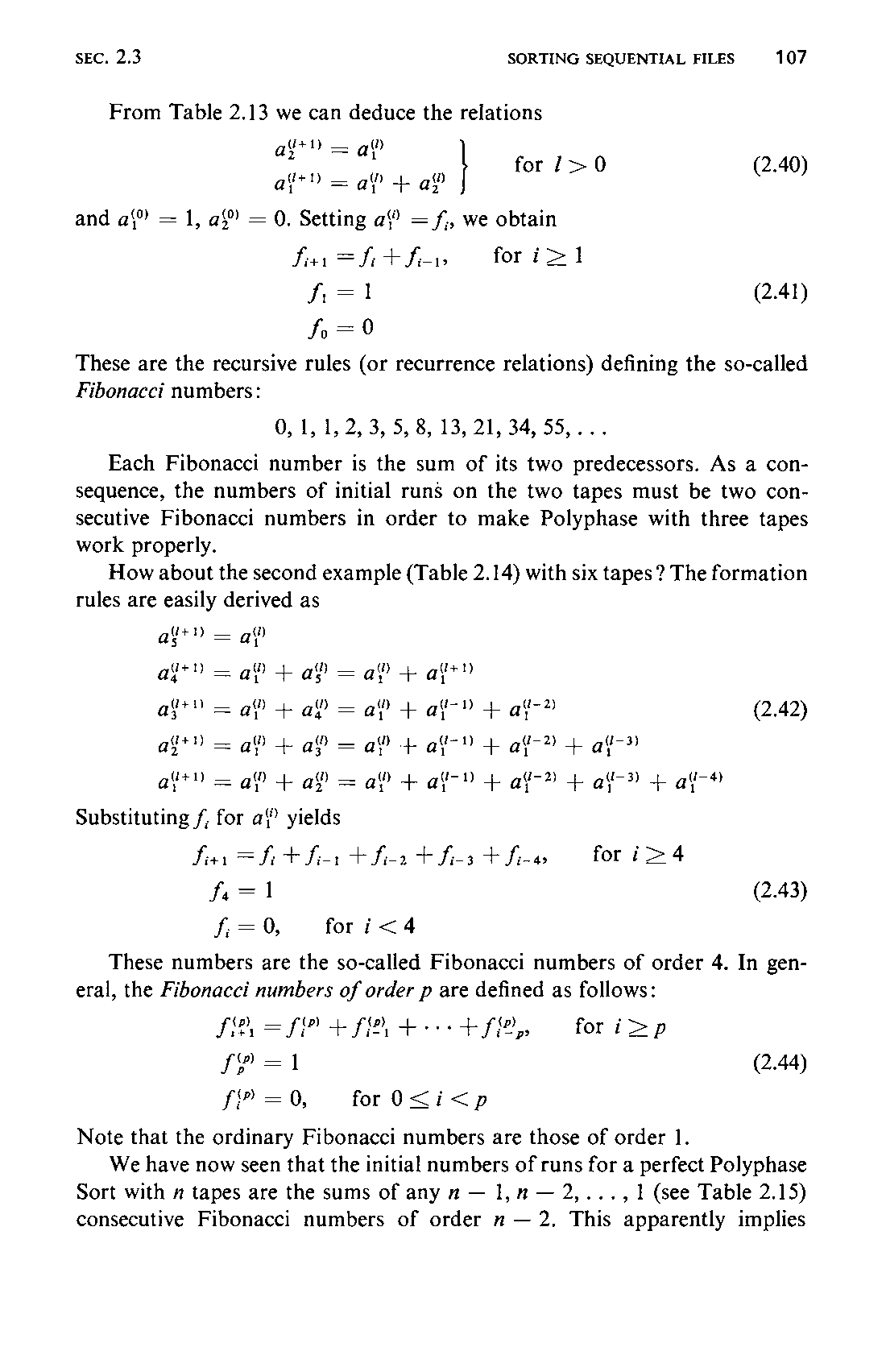
and $a_1^{(0)} = 1$, $a_2^{(0)} = 0$. Setting $a_1^{(i)} = f_i$, we obtain

These are the recursive rules (or recurrence relations) defining the so-called Fibonacci numbers:

Each Fibonacci number is the sum of its two predecessors. As a consequence, the numbers of initial runs on the two tapes must be two consecutive Fibonacci numbers in order to make Polyphase with three tapes work properly.

How about the second example (Table 2.14) with six tapes? The formation rules are easily derived as

Substituting $f_i$ for $a_1^{(i)}$ yields

These numbers are the so-called Fibonacci numbers of order 4. In general, the Fibonacci numbers of order $p$ are defined as follows:

Note that the ordinary Fibonacci numbers are those of order 1.

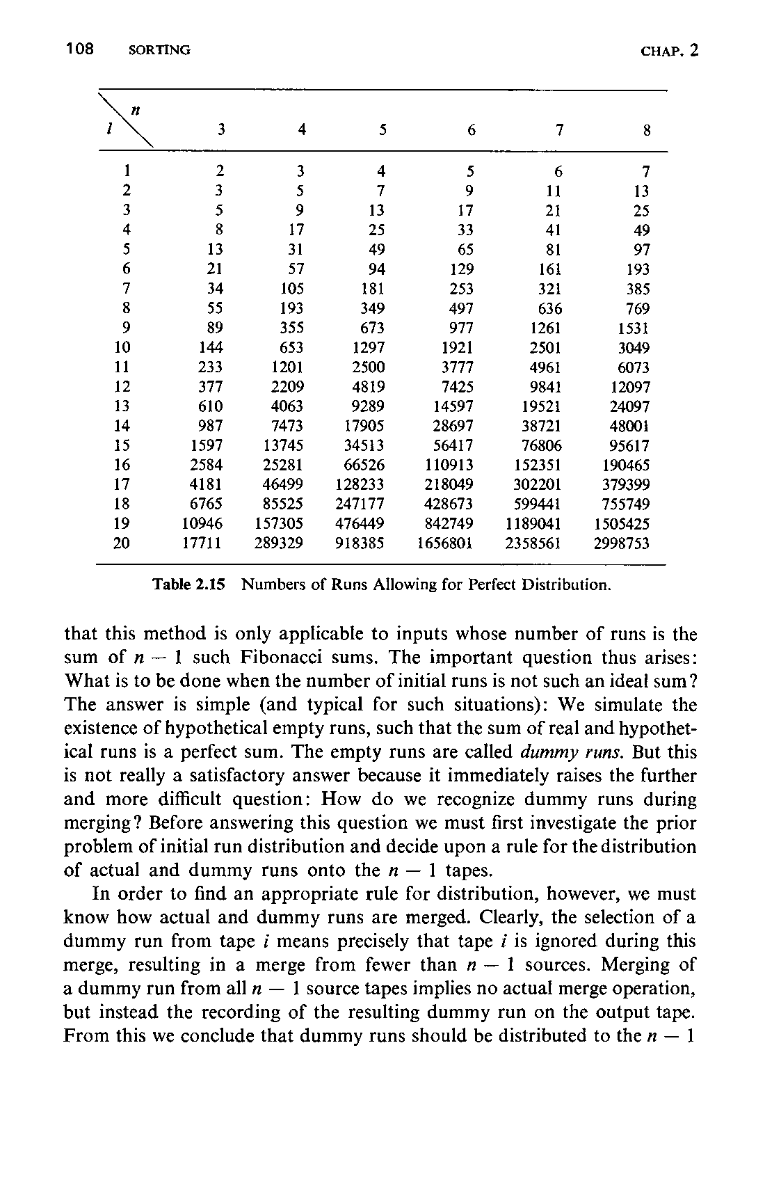
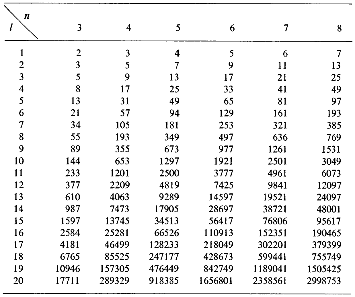
We have now seen that the initial numbers of runs for a perfect Polyphase Sort with $n$ tapes are the sums of any $n - 1, n - 2, \ldots, 1$ (see Table 2.15) consecutive Fibonacci numbers of order $n - 2$. This apparently implies108 that this method is only applicable to inputs whose number of runs is the sum of $n - 1$ such Fibonacci sums. The important question thus arises: What is to be done when the number of initial runs is not such an ideal sum? The answer is simple (and typical for such situations): We simulate the existence of hypothetical empty runs, such that the sum of real and hypothetical runs is a perfect sum. The empty runs are called dummy runs. But this is not really a satisfactory answer because it immediately raises the further and more difficult question: How do we recognize dummy runs during merging? Before answering this question we must first investigate the prior problem of initial run distribution and decide upon a rule for the distribution of actual and dummy runs onto the $n - 1$ tapes.

In order to find an appropriate rule for distribution, however, we must know how actual and dummy runs are merged. Clearly, the selection of a dummy run from tape $i$ means precisely that tape $i$ is ignored during this merge, resulting in a merge from fewer than $n - 1$ sources. Merging of a dummy run from all $n - 1$ source tapes implies no actual merge operation, but instead the recording of the resulting dummy run on the output tape. From this we conclude that dummy runs should be distributed to the $n - 1$109 tapes as uniformly as possible since we are interested in active merges from as many source tapes as possible.

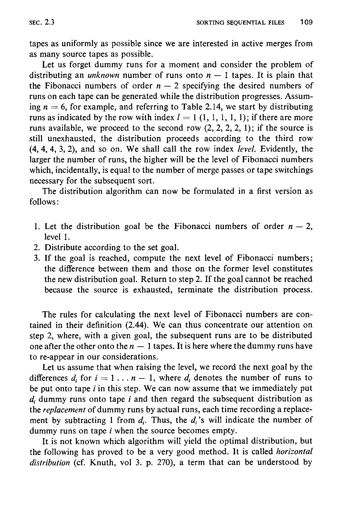
Let us forget dummy runs for a moment and consider the problem of distributing an unknown number of runs onto $n - 1$ tapes. It is plain that the Fibonacci numbers of order $n - 2$ specifying the desired numbers of runs on each tape can be generated while the distribution progresses. Assuming $n = 6$, for example, and referring to Table 2.14, we start by distributing runs as indicated by the row with index $l = 1$ (1, 1, 1, 1, 1); if there are more runs available, we proceed to the second row (2, 2, 2, 2, 1); if the source is still unexhausted, the distribution proceeds according to the third row (4, 4, 4, 3, 2), and so on. We shall call the row index level. Evidently, the larger the number of runs, the higher will be the level of Fibonacci numbers which, incidentally, is equal to the number of merge passes or tape switchings necessary for the subsequent sort.

The distribution algorithm can now be formulated in a first version as follows:

1. Let the distribution goal be the Fibonacci numbers of order $n - 2$, level 1.
2. Distribute according to the set goal.
3. If the goal is reached, compute the next level of Fibonacci numbers; the difference between them and those on the former level constitutes the new distribution goal. Return to step 2. If the goal cannot be reached because the source is exhausted, terminate the distribution process.

The rules for calculating the next level of Fibonacci numbers are contained in their definition (2.44). We can thus concentrate our attention on step 2, where, with a given goal, the subsequent runs are to be distributed one after the other onto the $n - 1$ tapes. It is here where the dummy runs have to re-appear in our considerations.

Let us assume that when raising the level, we record the next goal by the differences $d_i$ for $i = 1 \ldots n - 1$, where $d_i$ denotes the number of runs to be put onto tape $i$ in this step. We can now assume that we immediately put $d_i$ dummy runs onto tape $i$ and then regard the subsequent distribution as the replacement of dummy runs by actual runs, each time recording a replacement by subtracting 1 from $d_i$. Thus, the $d_i$’s will indicate the number of dummy runs on tape $i$ when the source becomes empty.

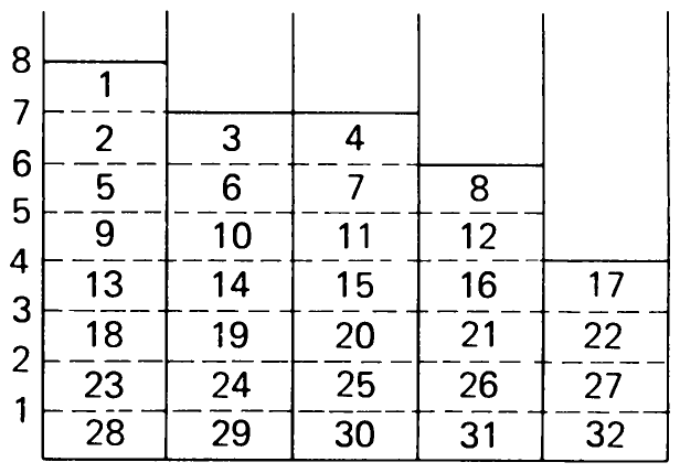
It is not known which algorithm will yield the optimal distribution, but the following has proved to be a very good method. It is called horizontal distribution (cf. Knuth, vol 3. p. 270), a term that can be understood by110 regarding the runs as being piled up in the form of silos, as shown in Fig. 2.16 for $n = 6$, level 5 (cf. Table 2.14).

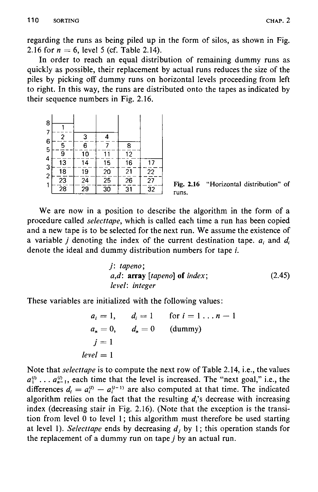
In order to reach an equal distribution of remaining dummy runs as quickly as possible, their replacement by actual runs reduces the size of the piles by picking off dummy runs on horizontal levels proceeding from left to right. In this way, the runs are distributed onto the tapes as indicated by their sequence numbers in Fig. 2.16.

We are now in a position to describe the algorithm in the form of a procedure called selecttape, which is called each time a run has been copied and a new tape is to be selected for the next run. We assume the existence of a variable $j$ denoting the index of the current destination tape. $a_i$ and $d_i$ denote the ideal and dummy distribution numbers for tape $i$.

j: tapeno;
a,d: array [tapeno] of index;
level: integer

These variables are initialized with the following values:

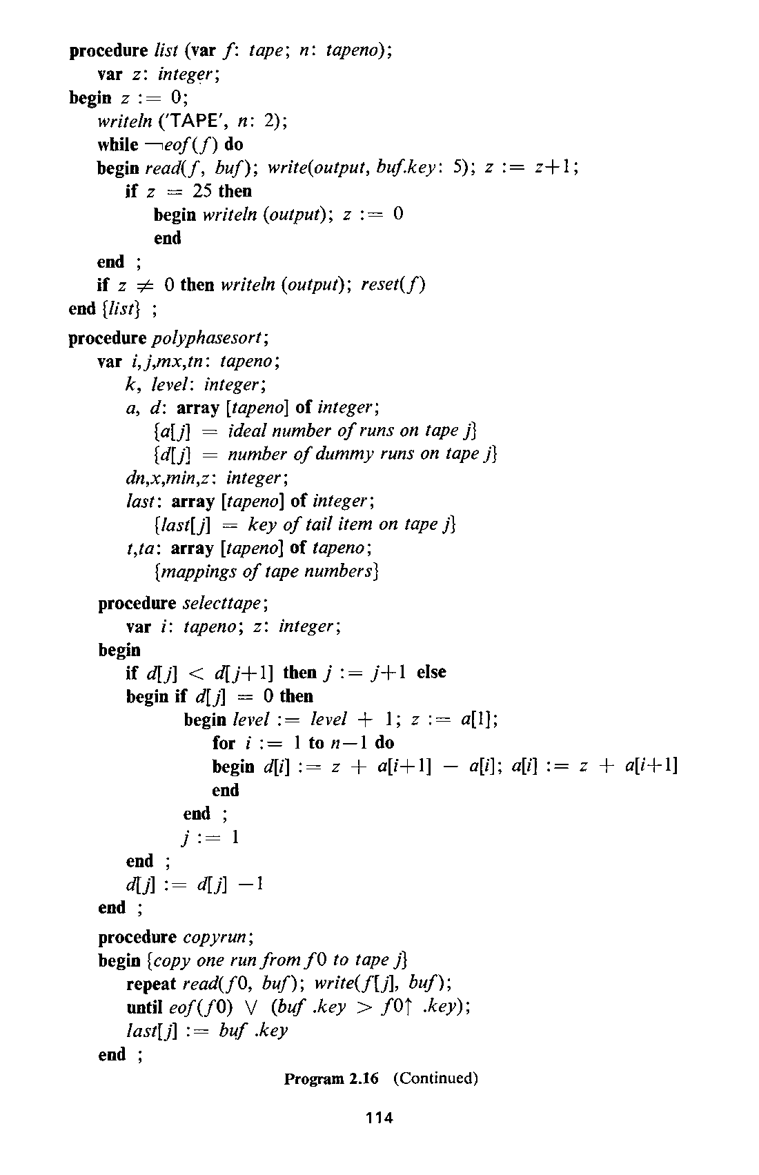
Note that selecttape is to compute the next row of Table 2.14, i.e., the values $a_1^{(l)} \ldots a_{n-1}^{(l)}$, each time that the level is increased. The “next goal,” i.e., the differences $d_i = a_i^{(l)} - a_i^{(l-1)}$ are also computed at that time. The indicated algorithm relies on the fact that the resulting $d_i$’s decrease with increasing index (decreasing stair in Fig. 2.16). (Note that the exception is the transition from level 0 to level 1; this algorithm must therefore be used starting at level 1). Selecttape ends by decreasing $d_j$ by 1; this operation stands for the replacement of a dummy run on tape $j$ by an actual run.

111

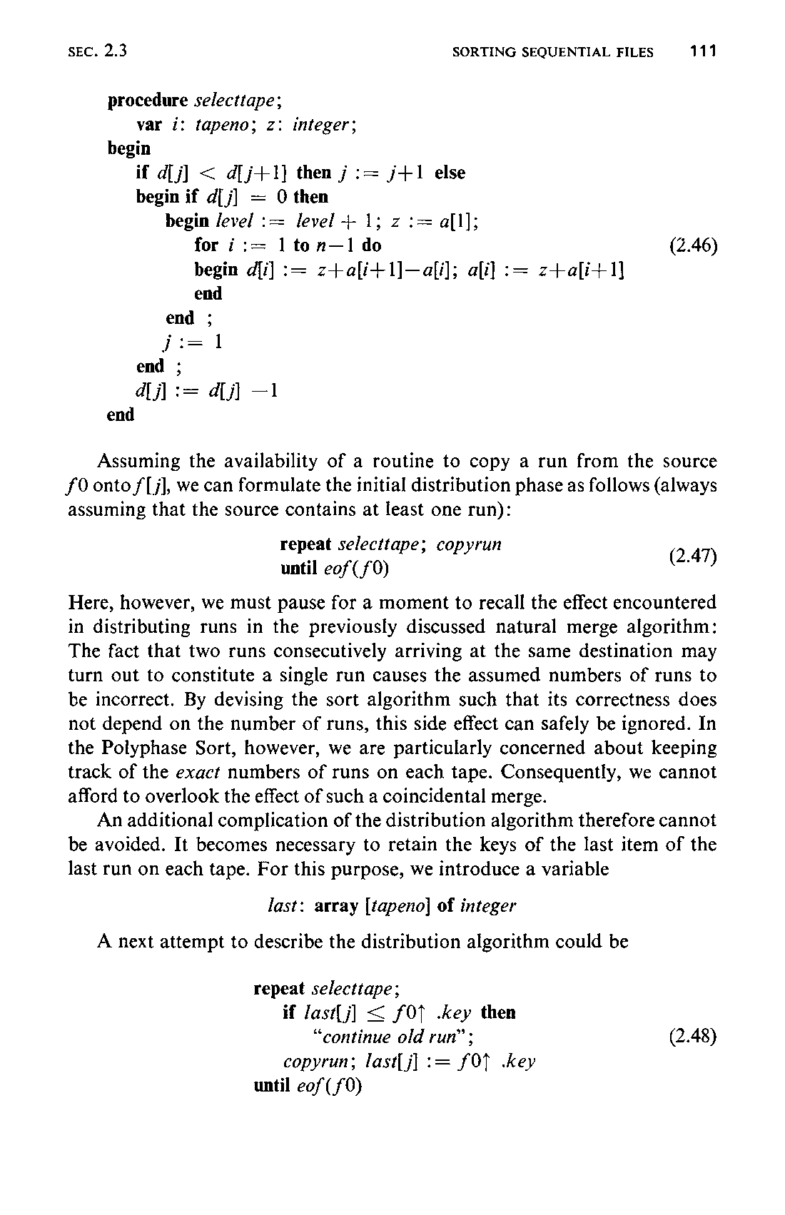
procedure selecttape;
   var i: tapeno; z: integer;
begin
   if d[j] < d[j+1] then j := j+1 else
   begin if d[j] = 0 then
      begin level := level + 1; z := a[1];
         for i := 1 to n-1 do
         begin d[i] := z+a[i+1]-a[i]; a[i] := z+a[i+1]
         end
      end ;
      j := 1
   end ;
   d[j] := d[j] -1
end

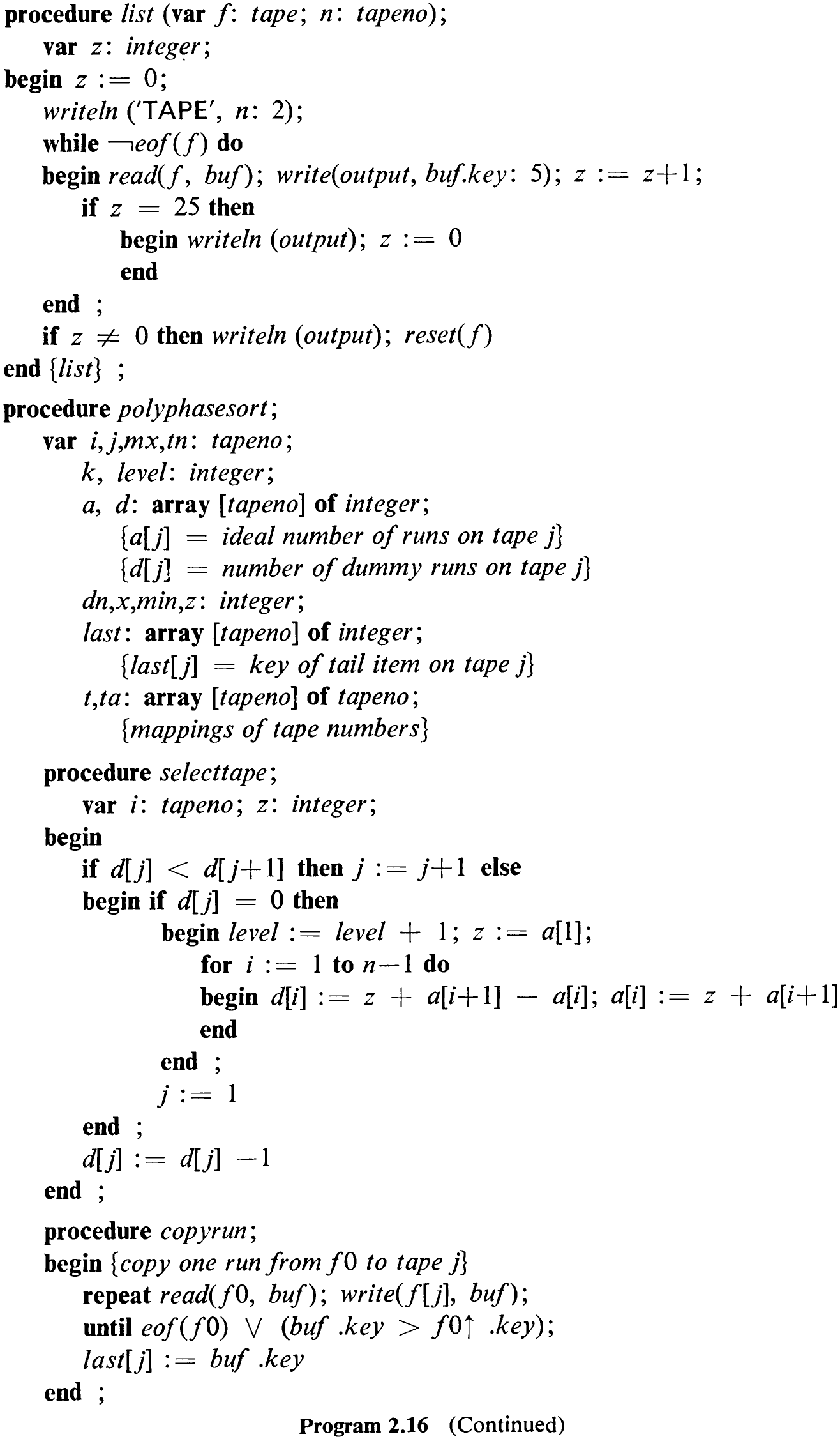
Assuming the availability of a routine to copy a run from the source f0 onto f[j], we can formulate the initial distribution phase as follows (always assuming that the source contains at least one run):

repeat selecttape; copyrun
until eof(f0)

Here, however, we must pause for a moment to recall the effect encountered in distributing runs in the previously discussed natural merge algorithm: The fact that two runs consecutively arriving at the same destination may turn out to constitute a single run causes the assumed numbers of runs to be incorrect. By devising the sort algorithm such that its correctness does not depend on the number of runs, this side effect can safely be ignored. In the Polyphase Sort, however, we are particularly concerned about keeping track of the exact numbers of runs on each tape. Consequently, we cannot afford to overlook the effect of such a coincidental merge.

An additional complication of the distribution algorithm therefore cannot be avoided. It becomes necessary to retain the keys of the last item of the last run on each tape. For this purpose, we introduce a variable

last: array [tapeno] of integer

A next attempt to describe the distribution algorithm could be

repeat selecttape;
   if last[j] ≤ f0↑.key then
      “continue old run”;
   copyrun; last[j] := f0↑.key
until eof(f0)

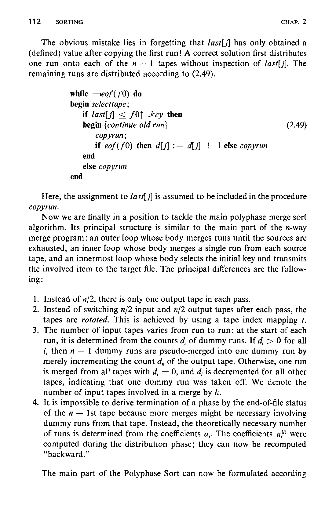
The obvious mistake lies in forgetting that /as¢[j] has only obtained a (defined) value after copying the first run! A correct solution first distributes one run onto each of the n — 1 tapes without inspection of /as¢{j]. The remaining runs are distributed according to (2.49).

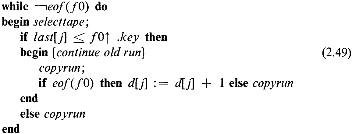
Here, the assignment to /ast[j] is assumed to be included in the procedure copyrun.

Now we are finally in a position to tackle the main polyphase merge sort algorithm. Its principal structure is similar to the main part of the n-way merge program: an outer loop whose body merges runs until the sources are exhausted, an inner loop whose body merges a single run from each source tape, and an innermost loop whose body selects the initial key and transmits the involved item to the target file. The principal differences are the following:

1. Instead of n/2, there is only one output tape in each pass.

2. Instead of switching n/2 input and n/2 output tapes after each pass, the tapes are rotated. This is achieved by using a tape index mapping t. 3. The number of input tapes varies from run to run; at the start of each run, it is determined from the counts d, of dummy runs. If d, > 0 for all i, then n — 1 dummy runs are pseudo-merged into one dummy run by merely incrementing the count d, of the output tape. Otherwise, one run is merged from all tapes with d, = 0, and d, is decremented for all other tapes, indicating that one dummy run was taken off. We denote the number of input tapes involved in a merge by k.

3. It is impossible to derive termination of a phase by the end-of-file status of the n — Ist tape because more merges might be necessary involving dummy runs from that tape. Instead, the theoretically necessary number of runs is determined from the coefficients a;. The coefficients a!” were computed during the distribution phase; they can now be recomputed “backward.”

The main part of the Polyphase Sort can now be formulated according113 to these rules, assuming that all » — 1 tapes with initial runs are reset and that the tape map is initially set to t; = i.

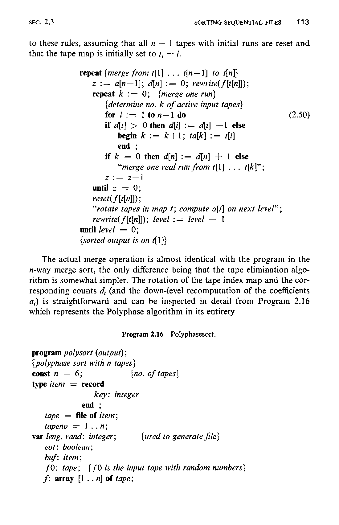
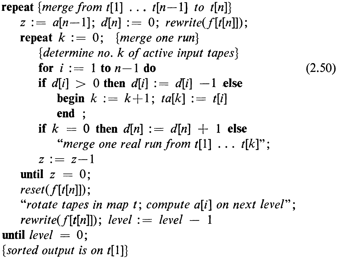
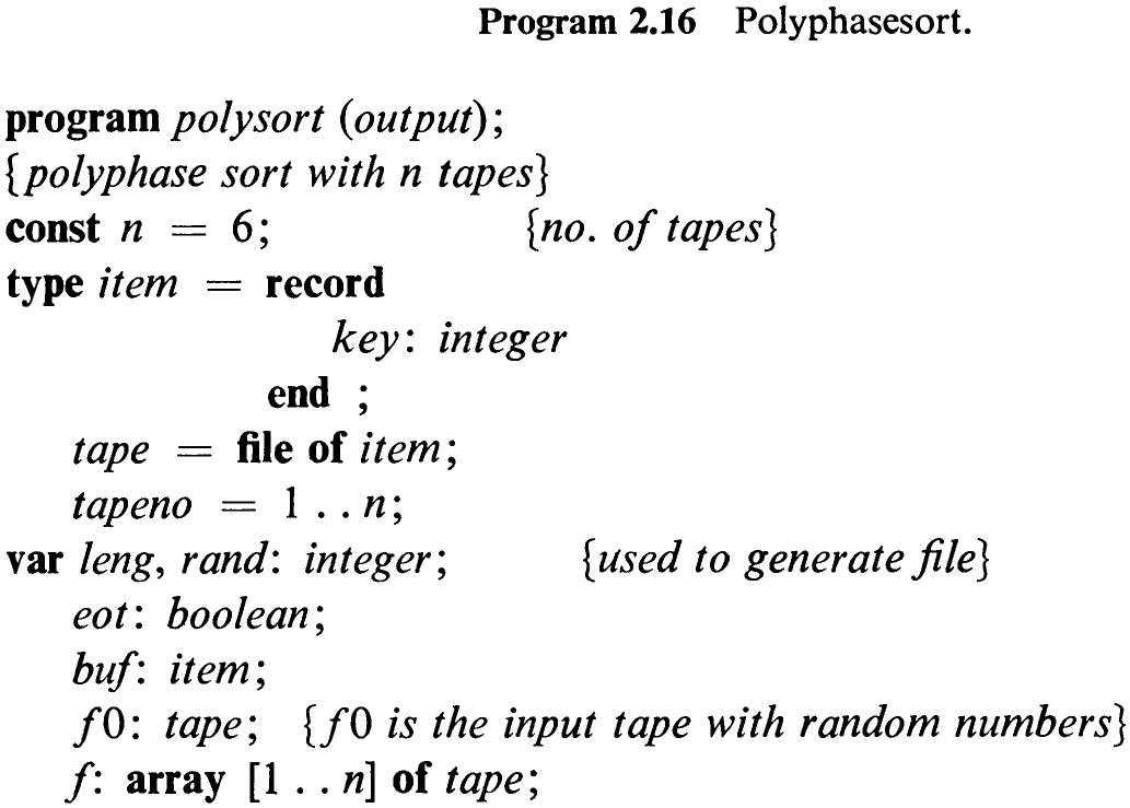
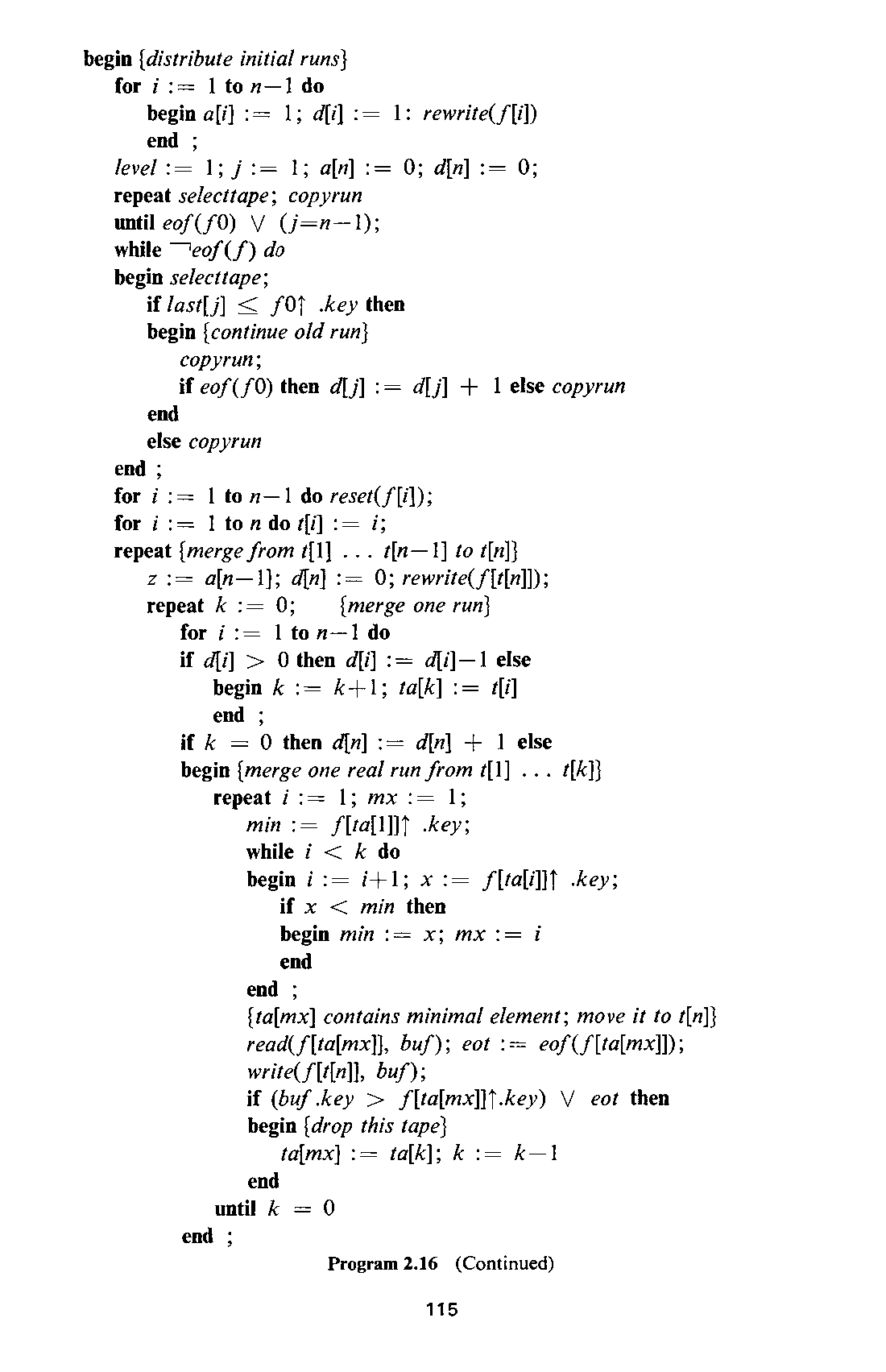
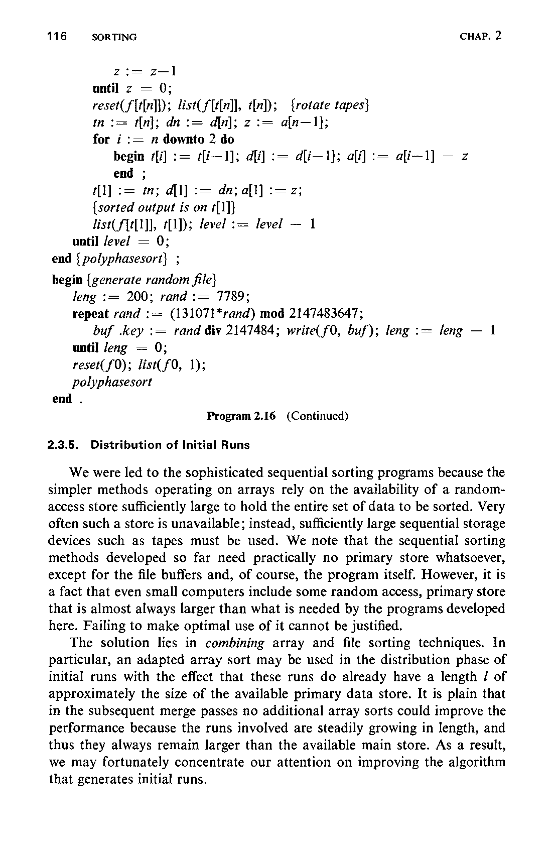
The actual merge operation is almost identical with the program in the n-way merge sort, the only difference being that the tape elimination algorithm is somewhat simpler. The rotation of the tape index map and the corresponding counts d, (and the down-level recomputation of the coefficients a,) is straightforward and can be inspected in detail from Program 2.16 which represents the Polyphase algorithm in its entirety

2.3.5 Distribution of Initial Runs

We were led to the sophisticated sequential sorting programs because the simpler methods operating on arrays rely on the availability of a random-access store sufficiently large to hold the entire set of data to be sorted. Very often such a store is unavailable; instead, sufficiently large sequential storage devices such as tapes must be used. We note that the sequential sorting methods developed so far need practically no primary store whatsoever, except for the file buffers and, of course, the program itself. However, it is a fact that even small computers include some random access, primary store that is almost always larger than what is needed by the programs developed here. Failing to make optimal use of it cannot be justified.

The solution lies in combining array and file sorting techniques. In particular, an adapted array sort may be used in the distribution phase of initial runs with the effect that these runs do already have a length / of approximately the size of the available primary data store. It is plain that in the subsequent merge passes no additional array sorts could improve the performance because the runs involved are steadily growing in length, and thus they always remain larger than the available main store. As a result, we may fortunately concentrate our attention on improving the algorithm that generates initial runs.

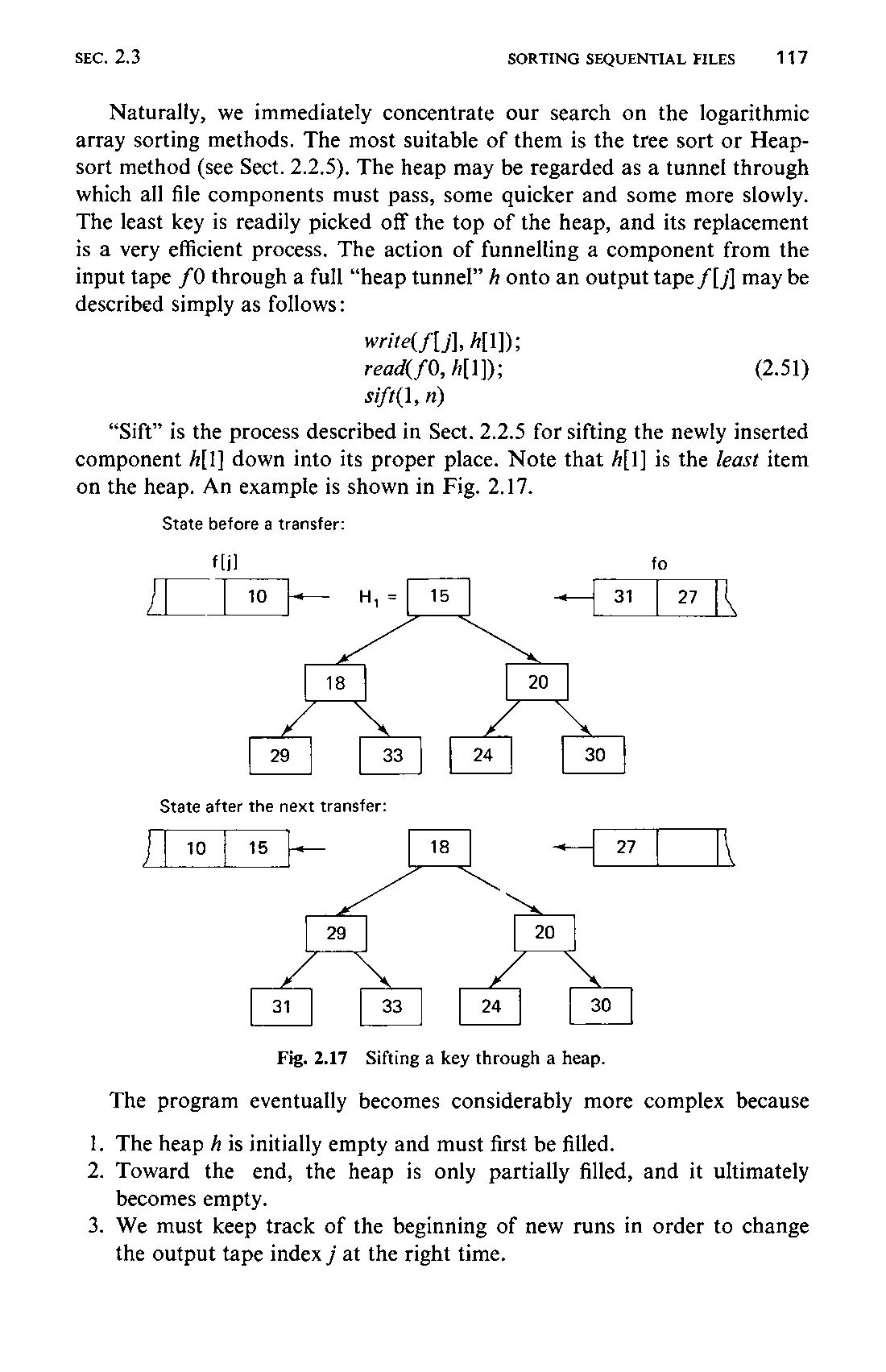
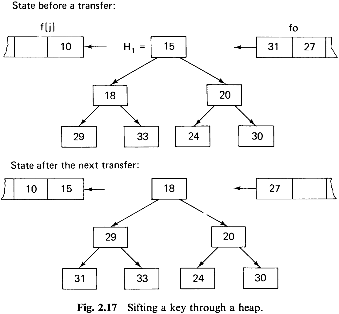
Naturally, we immediately concentrate our search on the logarithmic array sorting methods. The most suitable of them is the tree sort or Heapsort method (see Sect. 2.2.5). The heap may be regarded as a tunnel through which all file components must pass, some quicker and some more slowly. The least key is readily picked off the top of the heap, and its replacement is a very efficient process. The action of funnelling a component from the input tape f0 through a full “heap tunnel” / onto an output tape f[j/] may be described simply as follows:

“Sift” is the process described in Sect. 2.2.5 for sifting the newly inserted component A[1] down into its proper place. Note that A[1] is the /east item on the heap. An example is shown in Fig. 2.17.

The program eventually becomes considerably more complex because

1. The heap A is initially empty and must first be filled.

2. Toward the end, the heap is only partially filled, and it ultimately becomes empty.

3. We must keep track of the beginning of new runs in order to change the output tape index / at the right time.118 Before proceeding, let us formally declare the variables that are evidently involved in the game:

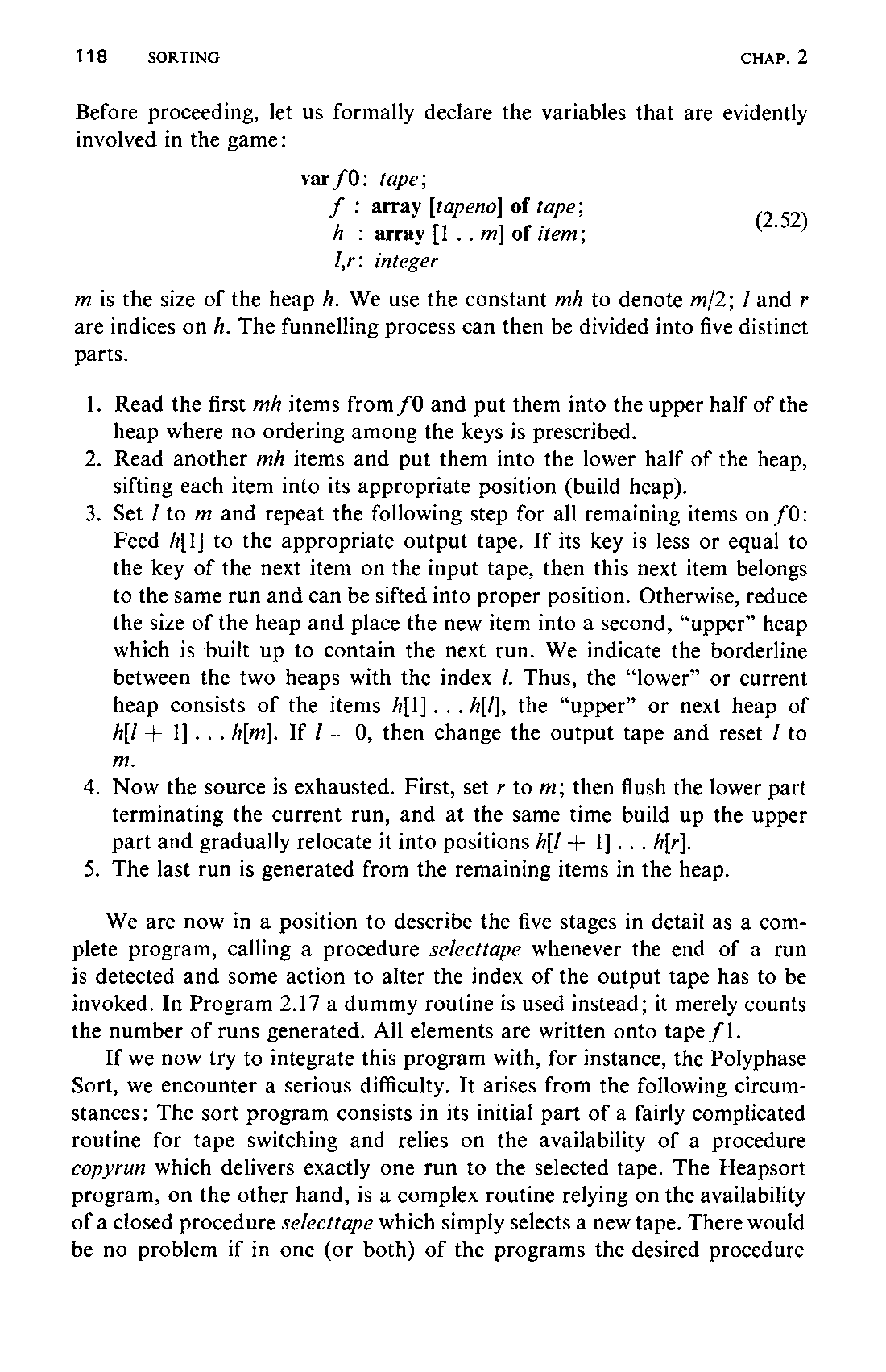
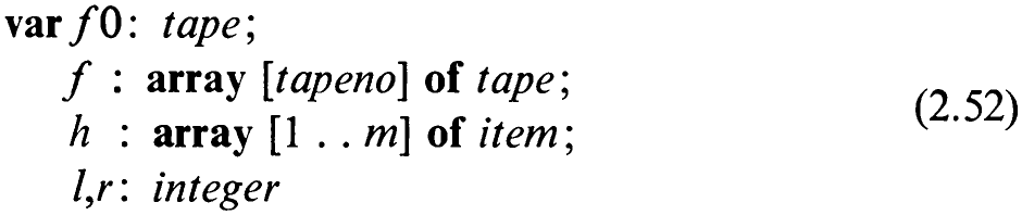
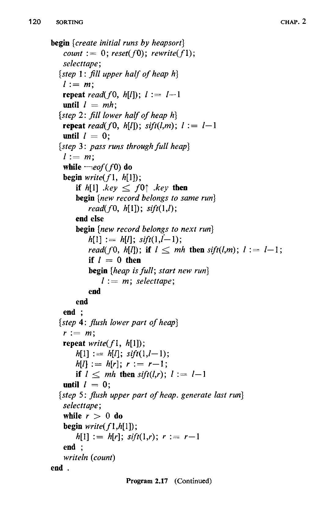
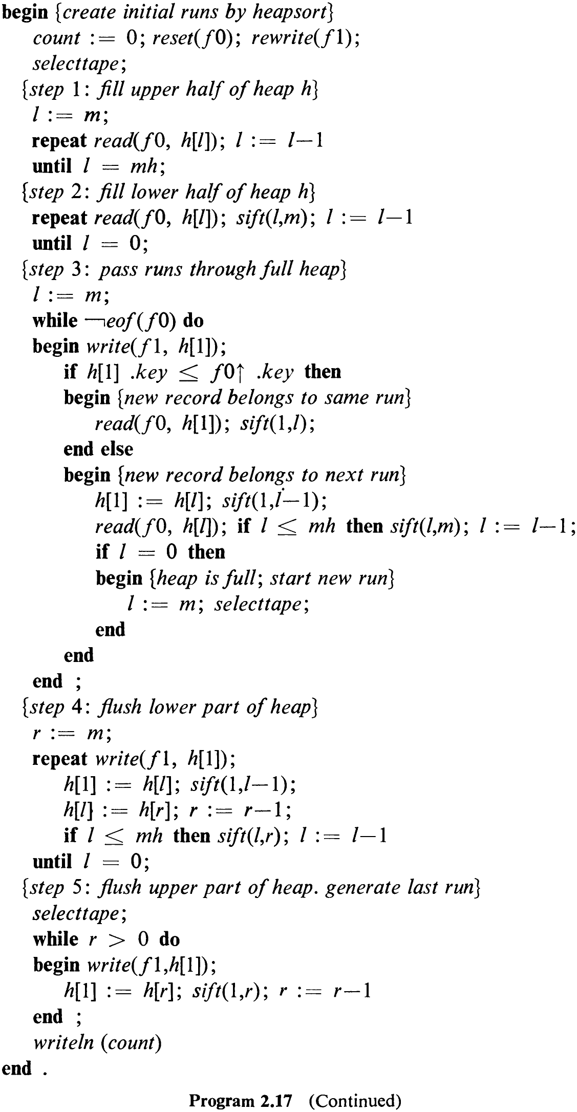
m is the size of the heap h. We use the constant mA to denote m/2; / and r are indices on h. The funnelling process can then be divided into five distinct parts.

1. Read the first mh items from f0 and put them into the upper half of the heap where no ordering among the keys is prescribed.

2. Read another mh items and put them into the lower half of the heap, sifting each item into its appropriate position (build heap).

3. Set / to m and repeat the following step for all remaining items on f0: Feed A[1] to the appropriate output tape. If its key is less or equal to the key of the next item on the input tape, then this next item belongs to the same run and can be sifted into proper position. Otherwise, reduce the size of the heap and place the new item into a second, “upper” heap which is ‘built up to contain the next run. We indicate the borderline between the two heaps with the index /. Thus, the “lower” or current heap consists of the items A[l]...A[/], the “upper” or next heap of Atl + 1]...A[m]. If 1 = 0, then change the output tape and reset / to

4. Now the source is exhausted. First, set r to m; then flush the lower part terminating the current run, and at the same time build up the upper part and gradually relocate it into positions A[/ + 1]... Afr].

5. The last run is generated from the remaining items in the heap.

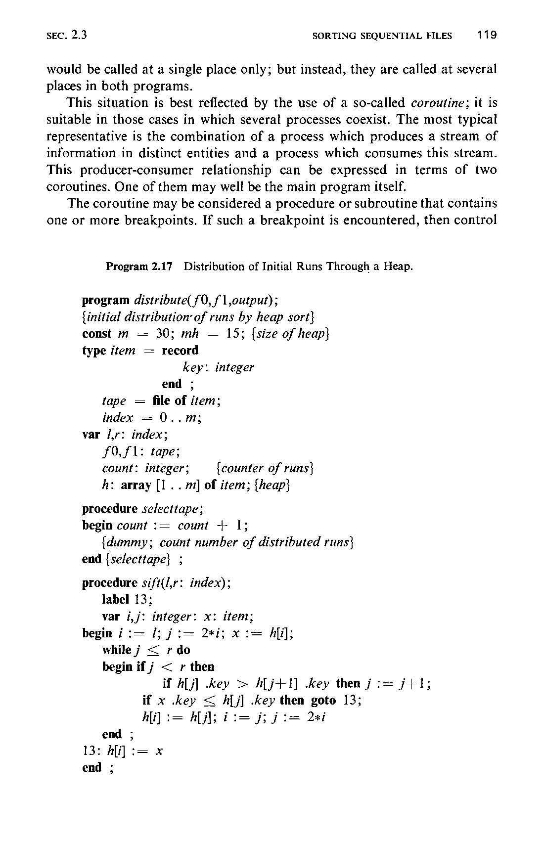
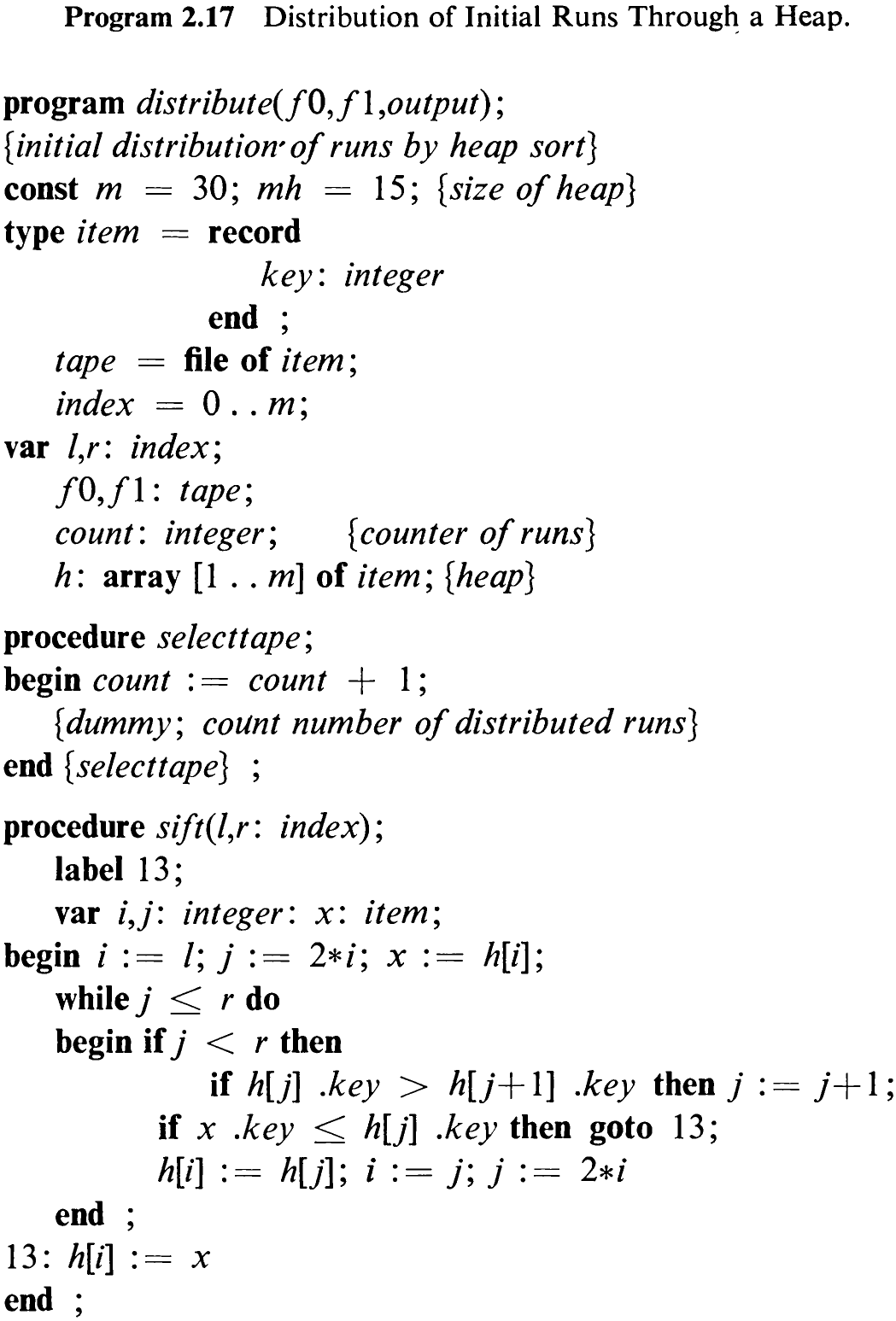
We are now in a position to describe the five stages in detail as a complete program, calling a procedure selecttape whenever the end of a run is detected and some action to alter the index of the output tape has to be invoked. In Program 2.17 a dummy routine is used instead; it merely counts the number of runs generated. All elements are written onto tape f1.

If we now try to integrate this program with, for instance, the Polyphase Sort, we encounter a serious difficulty. It arises from the following circumstances: The sort program consists in its initial part of a fairly complicated routine for tape switching and relies on the availability of a procedure copyrun which delivers exactly one run to the selected tape. The Heapsort program, on the other hand, is a complex routine relying on the availability of a closed procedure selecttape which simply selects a new tape. There would be no problem if in one (or both) of the programs the desired procedure119 would be called at a single place only; but instead, they are called at several places in both programs.

This situation is best reflected by the use of a so-called coroutine; it is suitable in those cases in which several processes coexist. The most typical representative is the combination of a process which produces a stream of information in distinct entities and a process which consumes this stream. This producer-consumer relationship can be expressed in terms of two coroutines. One of them may well be the main program itself.

The coroutine may be considered a procedure or subroutine that contains one or more breakpoints. If such a breakpoint is encountered, then control

returns to the program which had called the coroutine. Whenever the coroutine is called again, execution is resumed at that breakpoint. In our example we might consider the Polyphase Sort as the main program, calling upon copyrun which is formulated as a coroutine. It consists of the main body of Program 2.17 in which each call of selecttape now represents a breakpoint. The test for end of file would then have to be replaced systematically by a test of whether or not the coroutine had reached its endpoint. A logically sound formulation would be eoc(copyrun) in place of eof(f0).

Analysis and conclusions. What performance can be expected from a Polyphase Sort with initial distribution of runs by a Heapsort? We first discuss the improvement to be expected by introducing the heap.

In a sequence with randomly distributed keys the expected average length of runs is 2. What is this length after the sequence has been funnelled through a heap of size m? One is inclined to say m, but, fortunately, the actual result of probabilistic analysis is much better, namely, 2m (see Knuth, vol. 3, p. 254). Therefore, the expected improvement factor is m.

An estimate of the performance of Polyphase can be gathered from Table 2.15, indicating the maximal number of initial runs that can be sorted in a given number of partial passes (levels) with a given number n of tapes. As an example, with n = 6 tapes, and a heap of size m = 100, a file with up to 165,680,100 initial runs can be sorted within 20 partial passes. This is a remarkable performance.

Reviewing again the combination of Polyphase Sort and Heapsort, one cannot help but be amazed at the complexity of this program. After all, it performs the same easily defined task of re-ordering a set of items as is done by any of the short programs based on the straight array sorting principles. The moral of the entire chapter may be taken as an exhibition of the following:

1. The intimate connection between algorithm and underlying data structure and particularly the influence of the latter on the former.

2. The sophistication by which the performance of a program can be improved, even when the available structure for its data (sequence instead of array) is rather ill-suited for the task.