Sorting Arrays

The predominant requirement that has to be made for sorting methods on arrays is an economical use of the available store. This implies that the permutation of items which brings the items into order has to be performed in situ and that methods which transport items from an array $a$ to a result array $b$ are intrinsically of minor interest. Having thus restricted our choice of methods among the many possible solutions by the criterion of economy of storage, we proceed to a first classification according to their efficiency, i.e., their economy of time. A good measure of efficiency is obtained by counting the numbers $C$ of needed key comparisons and $M$ of moves (transpositions) of items. These numbers are functions of the number $n$ of items to be sorted. Whereas good sorting algorithms require in the order of $n \cdot \log n$ comparisons, we first discuss several simple and obvious sorting techniques, called straight methods, all of which require in the order $n^2$ comparisons of keys. There are three good reasons for presenting straight methods before proceeding to the faster algorithms.

1. Straight methods are particularly well-suited for elucidating the characteristics of the major sorting principles.
2. Their programs are easy to understand and are short. Remember that programs occupy storage as well!
3. Although sophisticated methods require fewer operations, these operations are usually more complex in their details; consequently, straight methods are faster for sufficiently small $n$, although they must not be used for large $n$.

Sorting methods which sort items in situ can be classified into three principal categories according to their underlying method:

1. Sorting by insertion.
2. Sorting by selection.
3. Sorting by exchange.

These three principles will now be examined and compared. The programs operate on the variable $a$ whose components are to be sorted in situ and refer to the data types item (2.2) and index, defined as

type index = 0..n;
var a: array[1..n] of item

2.2.1 Sorting by Straight Insertion

This method is widely used by card players. The items (cards) are conceptually divided into a destination sequence $a_1 \dots a_{i-1}$ and a source sequence $a_i \dots a_n$. In each step, starting with $i = 2$ and incrementing $i$ by unity, the $i$th element of the source sequence is picked and transferred into the destination sequence by inserting it at the appropriate place.

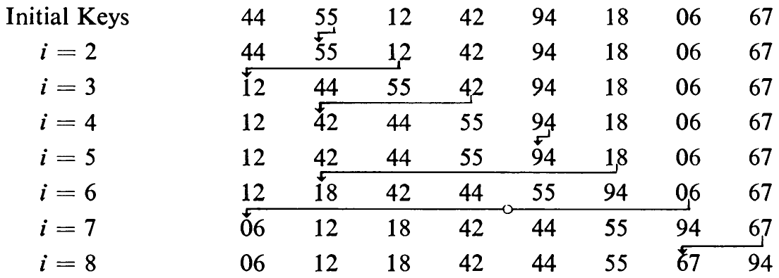
The process of sorting by insertion is shown in an example of eight numbers chosen at random (see Table 2.1). The algorithm of straight insertion is

for i := 2 to n do
   begin x := a[i];
      "insert x at the appropriate place in a₁ ... aᵢ"
   end

In the process of actually finding the appropriate place, it is convenient to alternate between comparisons and moves, i.e., to let $x$ “sift down” by comparing $x$ with the next item $a_j$, and either inserting $x$ or moving $a_j$ to the right and proceeding to the left. We note that there are two distinct conditions that may cause the termination of the “sifting down” process:

1. An item $a_j$ is found with a key less than the key of $x$.
2. The left end of the destination sequence is reached.

This typical case of a repetition with two termination conditions brings the well-known sentinel technique to our attention. It is easily applied to this case by posting a sentinel item $a_0 = x$. (Note that this must be included by extending the index range in the declaration of $a$ to 0..n.) The completed algorithm is formulated in Program 2.1.

procedure straightinsertion;
   var i,j: index;  x: item;
begin
   for i := 2 to n do
   begin x := a[i]; a[0] := x; j := i-1;
      while x.key < a[j].key do
         begin a[j+1] := a[j]; j := j-1;
         end ;
      a[j+1] := x
   end
end

Analysis of straight insertion. The number $C_i$ of key comparisons in the $i$th sift is at most $i - 1$, at least 1, and—assuming that all permutations of the $n$ keys are equally probable—$i/2$ in the average. The number $M_i$ of moves (assignments of items) is $C_i + 2$ (including the sentinel). Therefore, the total numbers of comparisons and moves are

The least numbers occur if the items are originally in order; the worst case occurs if the items are originally in reverse order. In this sense, sorting by insertion exhibits a truly natural behavior. It is plain that the given algorithm also describes a stable sorting process: it leaves the order of items with equal keys unchanged.

The algorithm of straight insertion is easily improved by noting that the destination sequence $a_1 \dots a_{i-1}$, in which the new item has to be inserted, is already ordered. Therefore, a faster method of determining the insertion point can be used. The obvious choice is a binary search that samples the destination sequence in the middle and continues bisecting until the insertion point is found. The modified sorting algorithm is called binary insertion, and is shown in Program 2.2.

procedure binaryinsertion;
   var i,j,l,r,m: index;  x: item;
begin
   for i := 2 to n do
   begin x := a[i]; l := 1; r := i-1;
      while l ≤ r do
      begin m := (l+r) div 2;
         if x.key < a[m].key then r := m-1 else l := m+1
      end ;
      for j := i-1 downto l do a[j+1] := a[j];
      a[l] := x;
   end
end

Analysis of binary insertion. The insertion position is found if $a_r.\mathit{key} \le x.\mathit{key} < a_1.\mathit{key}$. Thus, the search interval must in the end be 1; and this involves halving the interval of $i$ keys $\lceil \log_2 i \rceil$ times. Thus,

We approximate this sum by the integral

where $c = \log e = 1/\ln 2 = 1.44269 \dots$. The number of comparisons is essentially independent of the initial order of the items. However, because of the truncating character of the division involved in bisecting the search interval, the true number of comparisons needed with $i$ items may be up to 1 higher than expected. The nature of this bias is such that insertion positions at the low end are on the average located slightly faster than those at the high end, thereby favoring those cases in which the items are originally highly out of order. In fact, the minimum number of comparisons is needed if the items are initially in reverse order and the maximum if they are already in order. Hence, this is a case of unnatural behavior of a sorting algorithm.

Unfortunately, the improvement obtained by using a binary search method applies only to the number of comparisons but not to the number of necessary moves. In fact, since moving items, i.e., keys and associated information, is in general considerably more time-consuming than comparing two keys, the improvement is by no means drastic: the important term $M$ is still of the order $n^2$. And, in fact, re-sorting the already sorted array takes more time63 than does straight insertion with sequential search! This example demonstrates that an “obvious improvement” often has much less drastic consequences than one is first inclined to estimate and that in some cases (which do occur) the “improvement” may actually turn out to be a deterioration. After all, sorting by insertion does not appear to be a very suitable method for digital computers: insertion of an item with the subsequent shifting of an entire row of items by a single position is uneconomical. One should expect better results from a method in which moves of items are only performed upon single items and over longer distances. This idea leads to sorting by selection.

2.2.2 Sorting by Straight Selection

This method is based on the following principle:

1. Select the item with the least key.
2. Exchange it with the first item $a_1$.

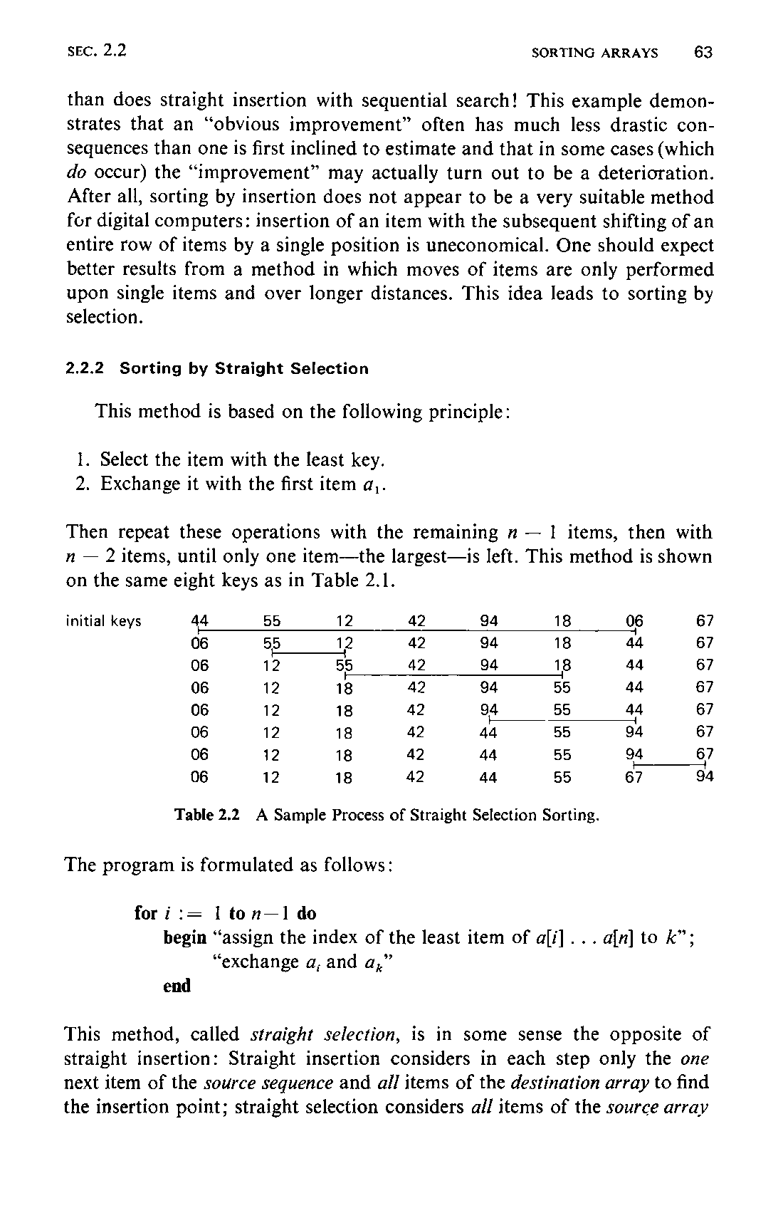
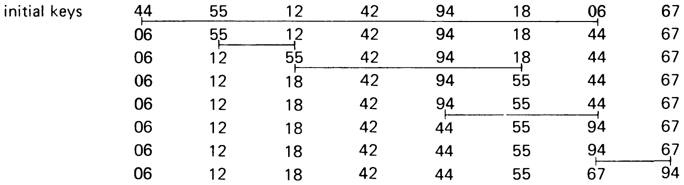
Then repeat these operations with the remaining $n - 1$ items, then with $n - 2$ items, until only one item—the largest—is left. This method is shown on the same eight keys as in Table 2.1.

The program is formulated as follows:

for i := 1 to n-1 do
   begin "assign the index of the least item of a[i] ... a[n] to k";
         "exchange aᵢ and aₖ"
   end

This method, called straight selection, is in some sense the opposite of straight insertion: Straight insertion considers in each step only the one next item of the source sequence and all items of the destination array to find the insertion point; straight selection considers all items of the source array64 to find the one with the least key and to deposit it as the one next item of the destination sequence. The entire program of straight selection is given in Program 2.3.

procedure straightselection;
   var i,j,k: index;  x: item;
begin for i := 1 to n-1 do
      begin k := i; x := a[i];
         for j := i+1 to n do
            if a[j].key < x.key then
            begin k := j; x := a[j]
            end ;
         a[k] := a[i]; a[i] := x;
      end
end

Analysis of straight selection. Evidently, the number $C$ of key comparisons is independent of the initial order of keys. In this sense, this method may be said to behave less naturally than straight insertion. We obtain

The number $M$ of moves is at least

in the case of initially ordered keys and at most

if initially the keys are in reverse order. The average $M_{\mathrm{ave}}$ is difficult to determine in spite of the algorithm’s simplicity. It depends on the number of times that $k_j$ is found to be less than all preceding numbers $k_1 \dots k_{j-1}$ when scanning a sequence of numbers $k_1 \dots k_n$. This value, averaged over all $n!$ permutations of $n$ keys is

where $H_n$ is the $n$th harmonic number

(cf. Knuth, Vol. 1, pp. 95–99).

$H_n$ can be expressed as

where $\gamma = 0.577216 \dots$ is Euler’s constant. For sufficiently large $n$, we may ignore the fractional terms and therefore approximate the average number of assignments in the $i$th pass as

The average number of moves $M_{\mathrm{ave}}$ in a selection sort is then the sum of $F_i$ with $i$ ranging from 1 to $n$.

By further approximating the sum of discrete terms by the integral

we obtain an approximate value

We may conclude that in general the algorithm of straight selection is to be preferred over straight insertion, although in the cases in which keys are initially sorted or almost sorted, straight insertion is still somewhat faster.

2.2.3 Sorting by Straight Exchange

The classification of a sorting method is seldom entirely clear-cut. Both previously discussed methods can also be viewed as exchange sorts. In this section, however, we present a method in which the exchange of two items is the dominant characteristic of the process. The subsequent algorithm of straight exchanging is based on the principle of comparing and exchanging pairs of adjacent items until all items are sorted.

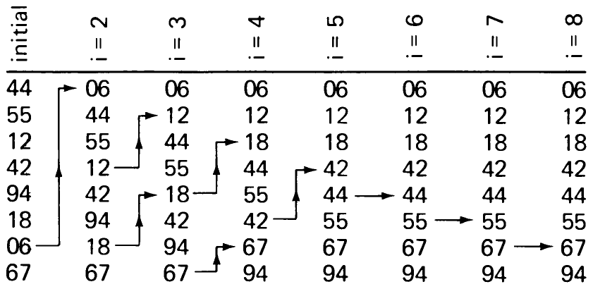
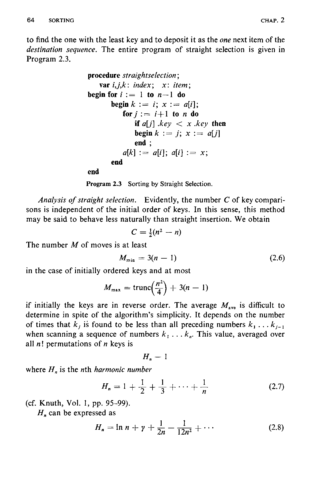
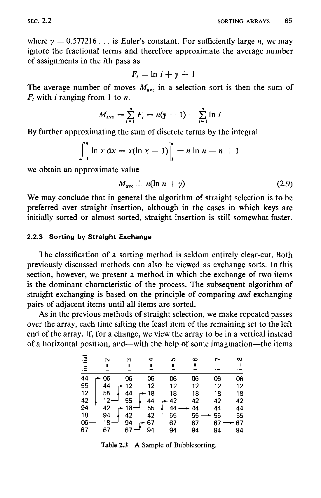
As in the previous methods of straight selection, we make repeated passes over the array, each time sifting the least item of the remaining set to the left end of the array. If, for a change, we view the array to be in a vertical instead of a horizontal position, and—with the help of some imagination—the items66 as bubbles in a water tank with “weights” according to their keys, then each pass over the array results in the ascension of a bubble to its appropriate level of weight (see Table 2.3). This method is widely known as the Bubblesort. Its simplest form is shown in Program 2.4.

procedure bubblesort;
   var i,j: index;  x: item;
begin for i := 2 to n do
      begin for j := n downto i do
               if a[j-1].key > a[j].key then
               begin x := a[j-1]; a[j-1] := a[j]; a[j] := x
               end
      end
end {bubblesort}

This algorithm easily lends itself to some improvements. The example in Table 2.3 shows that the last three passes have no effect on the order of the items because the items are already sorted. An obvious technique for improving this algorithm is to remember whether or not any exchange had taken place during a pass. A last pass without further exchange operations is therefore necessary to determine that the algorithm may be terminated. However, this improvement may itself be improved by remembering not merely the fact that an exchange took place, but rather the position (index) of the last exchange. For example, it is plain that all pairs of adjacent items below this index $k$ are in the desired order. Subsequent scans may therefore be terminated at this index instead of having to proceed to the predetermined lower limit $i$. The careful programmer will, however, notice a peculiar asymmetry: A single misplaced bubble in the “heavy” end of an otherwise sorted array will sift into order in a single pass, but a misplaced item in the “light” end will sink toward its correct position only one step in each pass. For example, the array

12  18  42  44  55  67  94  06

will be sorted by the improved Bubblesort in a single pass, but the array

94  06  12  18  42  44  55  67

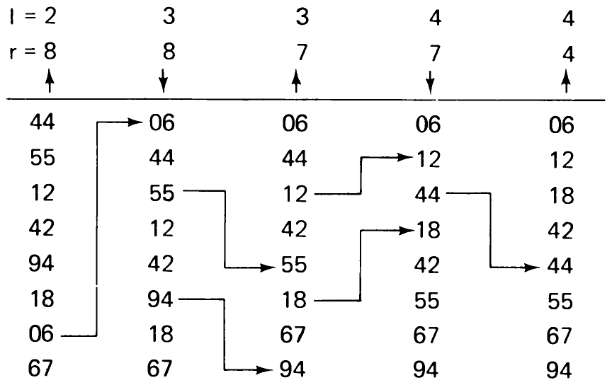
will require seven passes for sorting. This unnatural asymmetry suggests a third improvement: alternating the direction of consecutive passes. We appropriately call the resulting algorithm Shakersort. Its behavior is illustrated in Table 2.4 by applying it to the same eight keys that were used in Table 2.3.

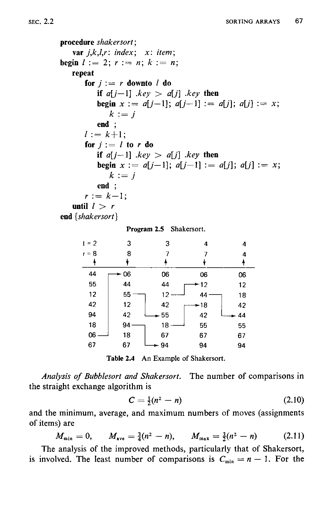
procedure shakersort;
   var j,k,l,r: index;  x: item;
begin l := 2; r := n; k := n;
   repeat
      for j := r downto l do
         if a[j-1].key > a[j].key then
         begin x := a[j-1]; a[j-1] := a[j]; a[j] := x;
            k := j
         end ;
      l := k+1;
      for j := l to r do
         if a[j-1].key > a[j].key then
         begin x := a[j-1]; a[j-1] := a[j]; a[j] := x;
            k := j
         end ;
      r := k-1;
   until l > r
end {shakersort}

Analysis of Bubblesort and Shakersort. The number of comparisons in the straight exchange algorithm is

and the minimum, average, and maximum numbers of moves (assignments of items) are

The analysis of the improved methods, particularly that of Shakersort, is involved. The least number of comparisons is $C_{\mathrm{min}} = n - 1$. For the68 improved Bubblesort, Knuth arrives at an average number of passes proportional to $n - k_1\sqrt{n}$, and an average number of comparisons proportional to $\tfrac{1}{2}[n^2 - n(k_2 + \ln n)]$. But we note that all improvements mentioned above do in no way affect the number of exchanges; they only reduce the number of redundant double checks. Unfortunately, an exchange of two items is generally a much more costly operation than a comparison of keys; our clever improvements therefore have a much less profound effect than one would intuitively expect.

This analysis shows that the exchange sort and its minor improvements are inferior to both the insertion and the selection sorts; and in fact, the Bubblesort has hardly anything to recommend it except its catchy name. The Shakersort algorithm is used with advantage in those cases in which it is known that the items are already almost in order—a rare case in practice.

It can be shown that the average distance that each of the $n$ items has to travel during a sort is $n/3$ places. This figure provides a clue in the search for improved, i.e., more effective sorting methods. All straight sorting methods essentially move each item by one position in each elementary step. Therefore, they are bound to require in the order $n^2$ such steps. Any improvement must be based on the principle of moving items over greater distances in single leaps.

Subsequently, three improved methods will be discussed, namely, one for each basic sorting method: insertion, selection, and exchange.

2.2.4 Insertion Sort by Diminishing Increment

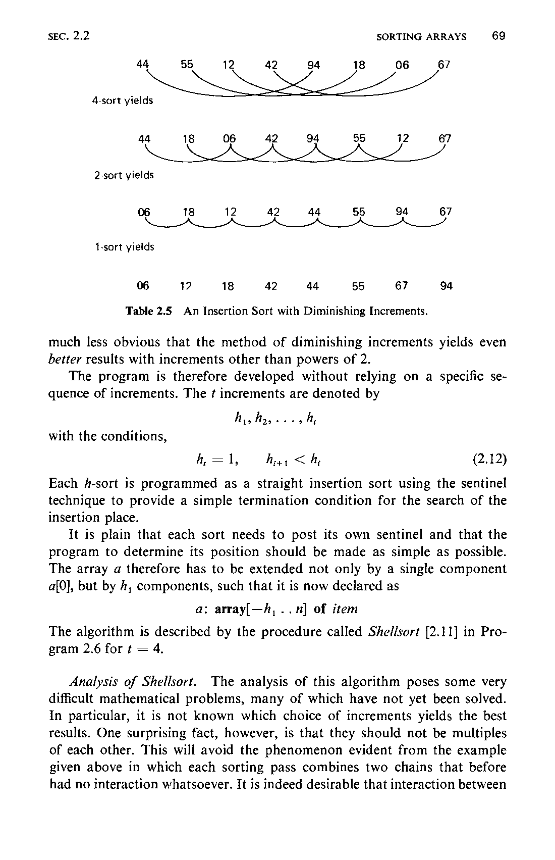
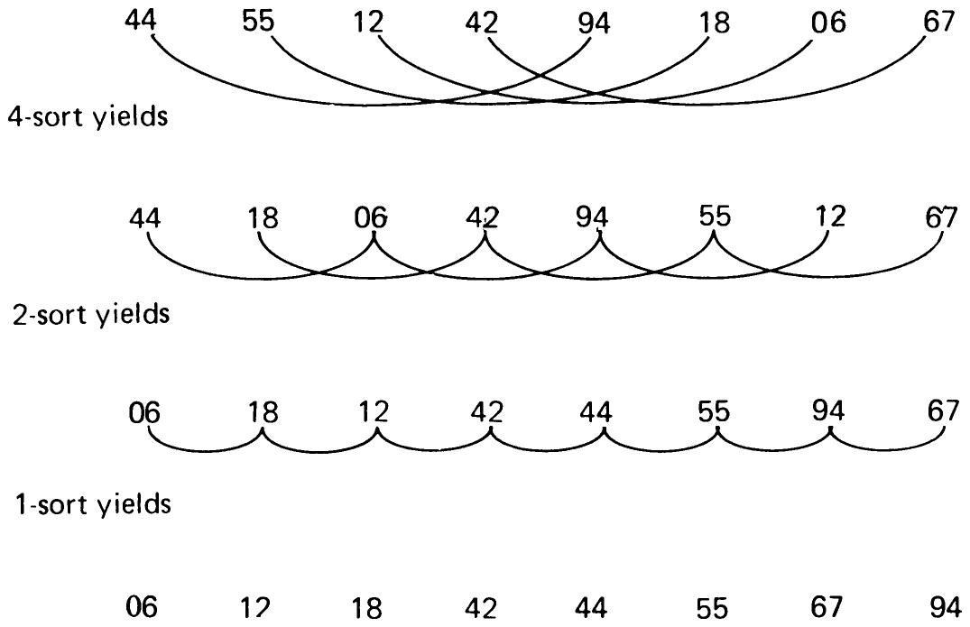
A refinement of the straight insertion sort was proposed by D. L. Shell in 1959. The method is explained and demonstrated on our standard example of eight items (see Table 2.5). First, all items which are four positions apart are grouped and sorted separately. This process is called a 4-sort. In this example of eight items, each group contains exactly two items. After this first pass, the items are regrouped into groups with items two positions apart and then sorted anew. This process is called a 2-sort. Finally, in a third pass, all items are sorted in an ordinary sort or 1-sort.

One may at first wonder if the necessity of several sorting passes, each of which involves all items, will not introduce more work than it saves. However, each sorting step over a chain involves either relatively few items or the items are already quite well ordered and comparatively few re-arrangements are required.

It is obvious that the method results in an ordered array, and it is fairly obvious that each pass will profit from previous passes (since each $i$-sort combines two groups sorted in the preceding $2i$-sort). It is also obvious that any sequence of increments will be acceptable, as long as the last one is unity, because in the worst case the last pass will do all the work. It is, however,69 much less obvious that the method of diminishing increments yields even better results with increments other than powers of 2.

The program is therefore developed without relying on a specific sequence of increments. The $t$ increments are denoted by

with the conditions,

Each $h$-sort is programmed as a straight insertion sort using the sentinel technique to provide a simple termination condition for the search of the insertion place.

It is plain that each sort needs to post its own sentinel and that the program to determine its position should be made as simple as possible. The array $a$ therefore has to be extended not only by a single component a[0], but by $h_1$ components, such that it is now declared as

a: array[-h₁..n] of item

The algorithm is described by the procedure called Shellsort [2.11] in Program 2.6 for $t = 4$.

Analysis of Shellsort. The analysis of this algorithm poses some very difficult mathematical problems, many of which have not yet been solved. In particular, it is not known which choice of increments yields the best results. One surprising fact, however, is that they should not be multiples of each other. This will avoid the phenomenon evident from the example given above in which each sorting pass combines two chains that before had no interaction whatsoever. It is indeed desirable that interaction between 70various chains takes place as often as possible, and the following theorem holds:

If a $k$-sorted sequence is $i$-sorted, then it remains $k$-sorted.

procedure shellsort;
  const t = 4;
  var i,j,k,s: index;  x: item; m: 1 .. t;
    h: array [1 .. t] of integer;
begin h[1] := 9; h[2] := 5; h[3] := 3; h[4] := 1;
  for m := 1 to t do
  begin k := h[m]; s := -k; {sentinel position}
    for i := k+1 to n do
    begin x := a[i]; j := i-k;
      if s=0 then s := -k; s := s+1; a[s] := x;
      while x .key < a[j] .key do
      begin a[j+k] := a[j]; j := j-k
      end ;
      a[j+k] := x
    end
  end
end

Knuth [2.8] indicates evidence that a reasonable choice of increments is the sequence (written in reverse order)

where $h_{k-1} = 3h_k + 1$, $h_t = 1$, and $t = \lfloor \log_3 n \rfloor - 1$. He also recommends the sequence

where $h_{k-1} = 2h_k + 1$, $h_t = 1$, and $t = \lfloor \log_2 n \rfloor - 1$. For the latter choice, mathematical analysis yields an effort proportional to $n^{1.2}$ required for sorting $n$ items with the Shellsort algorithm. Although this is a significant improvement over $n^2$, we will not expound further on this method, since even better algorithms are known.

2.2.5 Tree Sort

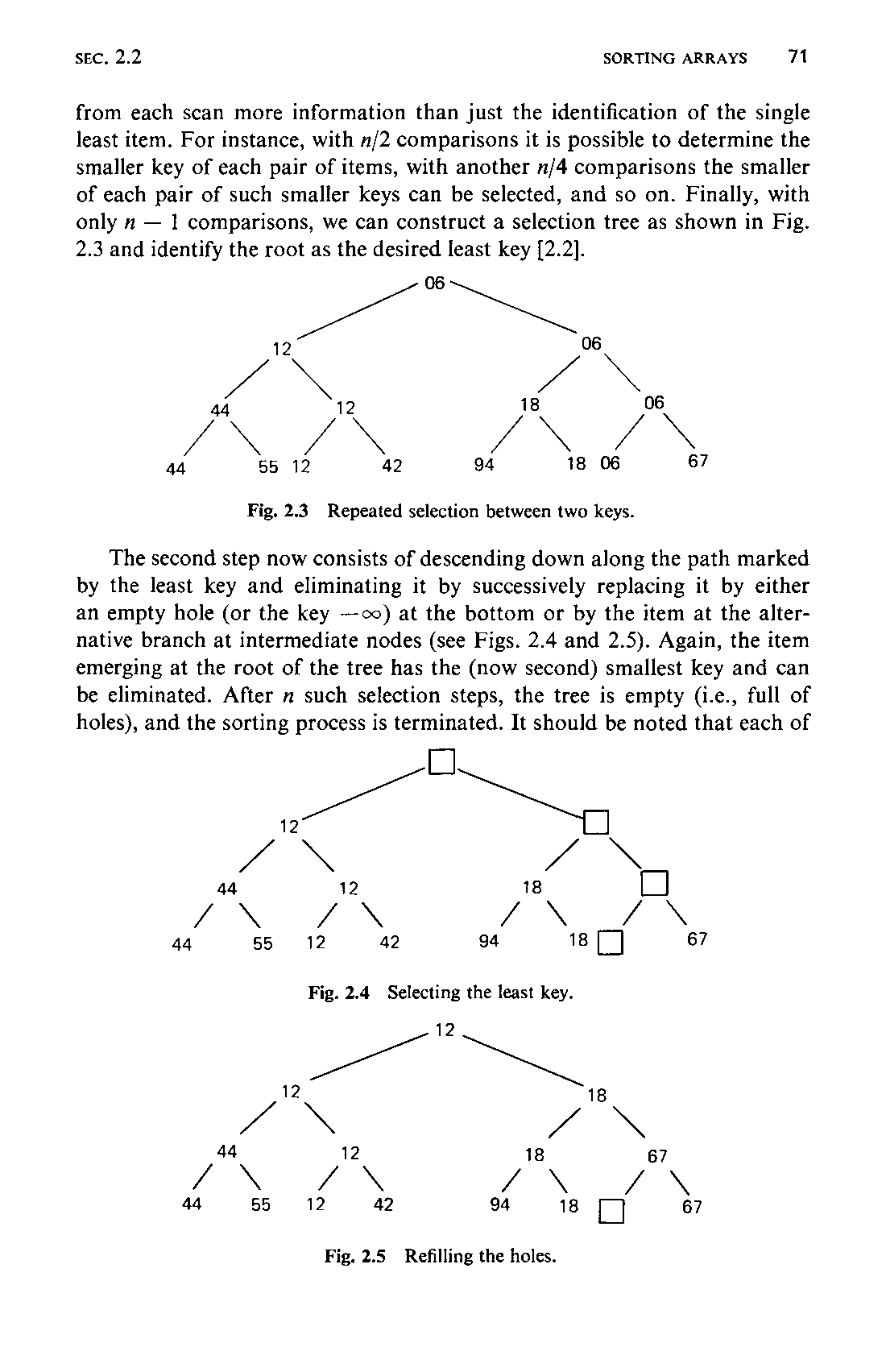
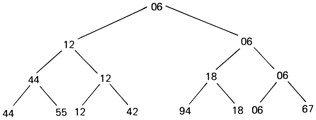
The method of sorting by straight selection is based on the repeated selection of the least key among $n$ items, among the remaining $n - 1$ items, etc. Clearly, finding the least key among $n$ items requires $n - 1$ comparisons, and finding it among $n - 1$ items needs $n - 2$ comparisons. So how can this selection sort possibly be improved? It can only be improved by retaining71 from each scan more information than just the identification of the single least item. For instance, with $n/2$ comparisons it is possible to determine the smaller key of each pair of items, with another $n/4$ comparisons the smaller of each pair of such smaller keys can be selected, and so on. Finally, with only $n - 1$ comparisons, we can construct a selection tree as shown in Fig. 2.3 and identify the root as the desired least key [2.2].

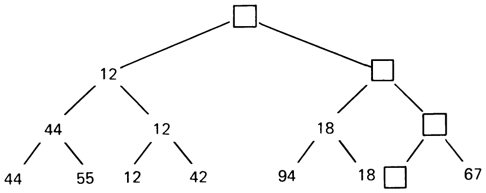
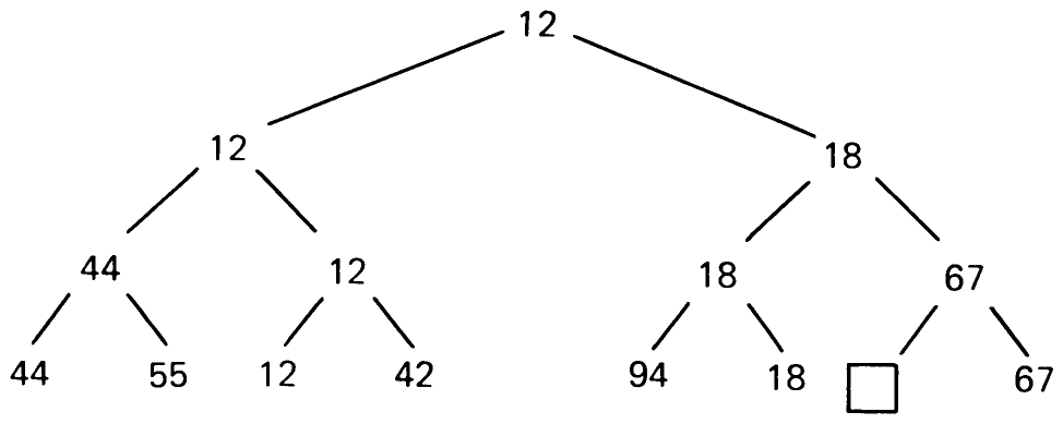
The second step now consists of descending down along the path marked by the least key and eliminating it by successively replacing it by either an empty hole (or the key $-\infty$) at the bottom or by the item at the alternative branch at intermediate nodes (see Figs. 2.4 and 2.5). Again, the item emerging at the root of the tree has the (now second) smallest key and can be eliminated. After $n$ such selection steps, the tree is empty (i.e., full of holes), and the sorting process is terminated. It should be noted that each of72 the $n$ selection steps requires only $\log_2 n$ comparisons. Therefore, the total selection process requires only on the order of $n \cdot \log n$ elementary operations in addition to the $n$ steps required by the construction of the tree. This is a very significant improvement over the straight methods requiring $n^2$ steps, and even over Shellsort that requires $n^{1.2}$ steps.

Naturally, the task of bookkeeping has become more elaborate, and therefore the complexity of individual steps is greater in the tree sort method; after all, in order to retain the increased amount of information gained from the initial pass, some sort of tree structure has to be created. Our next task is to find methods of organizing this information efficiently.

Of course, it would seem particularly desirable to eliminate the need for the holes ($-\infty$) that in the end populate the entire tree and are the source of many unnecessary comparisons. Moreover, a way should be found to represent the tree of $n$ items in $n$ units of storage, instead of in $2n - 1$ units as shown above. These goals are indeed achieved by a method called Heapsort by its inventor J. Williams [2-14]; it is plain that this method represents a drastic improvement over more conventional tree sorting approaches.

A heap is defined as a sequence of keys

such that

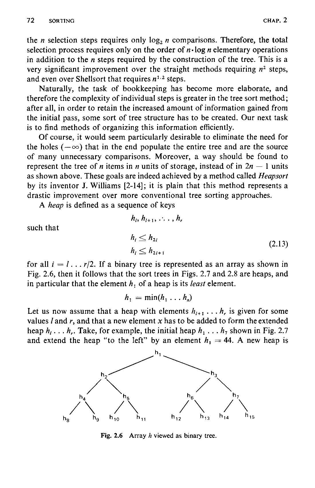
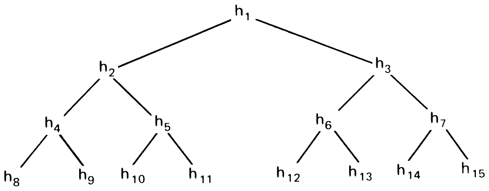
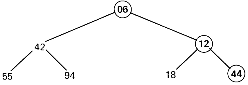
for all $i = l \dots r/2$. If a binary tree is represented as an array as shown in Fig. 2.6, then it follows that the sort trees in Figs. 2.7 and 2.8 are heaps, and in particular that the element $h_1$ of a heap is its least element.

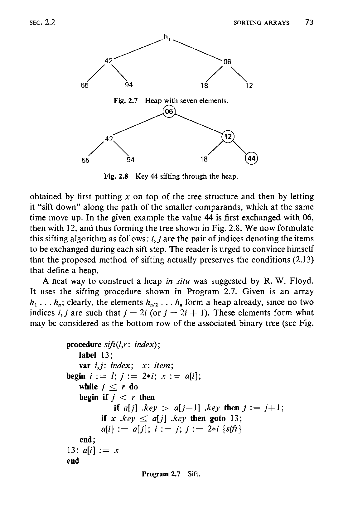
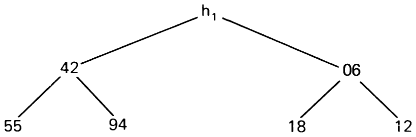
Let us now assume that a heap with elements $h_{l+1} \dots h_r$ is given for some values $l$ and $r$, and that a new element $x$ has to be added to form the extended heap $h_l \dots h_r$. Take, for example, the initial heap $h_1 \dots h_7$ shown in Fig. 2.7 and extend the heap “to the left” by an element $h_1 = 44$. A new heap is73 obtained by first putting $x$ on top of the tree structure and then by letting it “sift down” along the path of the smaller comparands, which at the same time move up. In the given example the value 44 is first exchanged with 06, then with 12, and thus forming the tree shown in Fig. 2.8. We now formulate this sifting algorithm as follows: $i$, $j$ are the pair of indices denoting the items to be exchanged during each sift step. The reader is urged to convince himself that the proposed method of sifting actually preserves the conditions (2.13) that define a heap.

procedure sift(l,r: index);
  label 13;
  var i,j: index;  x: item;
begin i := l; j := 2*i; x := a[i];
  while j ≤ r do
  begin if j < r then
          if a[j] .key > a[j+1] .key then j := j+1;
        if x .key ≤ a[j] .key then goto 13;
        a[i] := a[j]; i := j; j := 2*i {sift}
  end;
13: a[i] := x
end

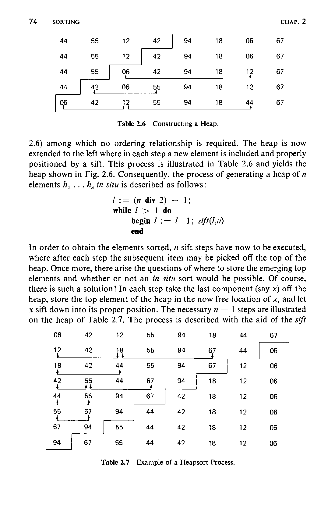
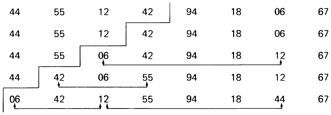
A neat way to construct a heap in situ was suggested by R. W. Floyd. It uses the sifting procedure shown in Program 2.7. Given is an array $h_1 \dots h_n$; clearly, the elements $h_{n/2} \dots h_n$ form a heap already, since no two indices $i$, $j$ are such that $j = 2i$ (or $j = 2i + 1$). These elements form what may be considered as the bottom row of the associated binary tree (see Fig.74 2.6) among which no ordering relationship is required. The heap is now extended to the left where in each step a new element is included and properly positioned by a sift. This process is illustrated in Table 2.6 and yields the heap shown in Fig. 2.6. Consequently, the process of generating a heap of $n$ elements $h_1 \dots h_n$ in situ is described as follows:

l := (n div 2) + 1;
while l > 1 do
   begin l := l-1; sift(l,n)
   end

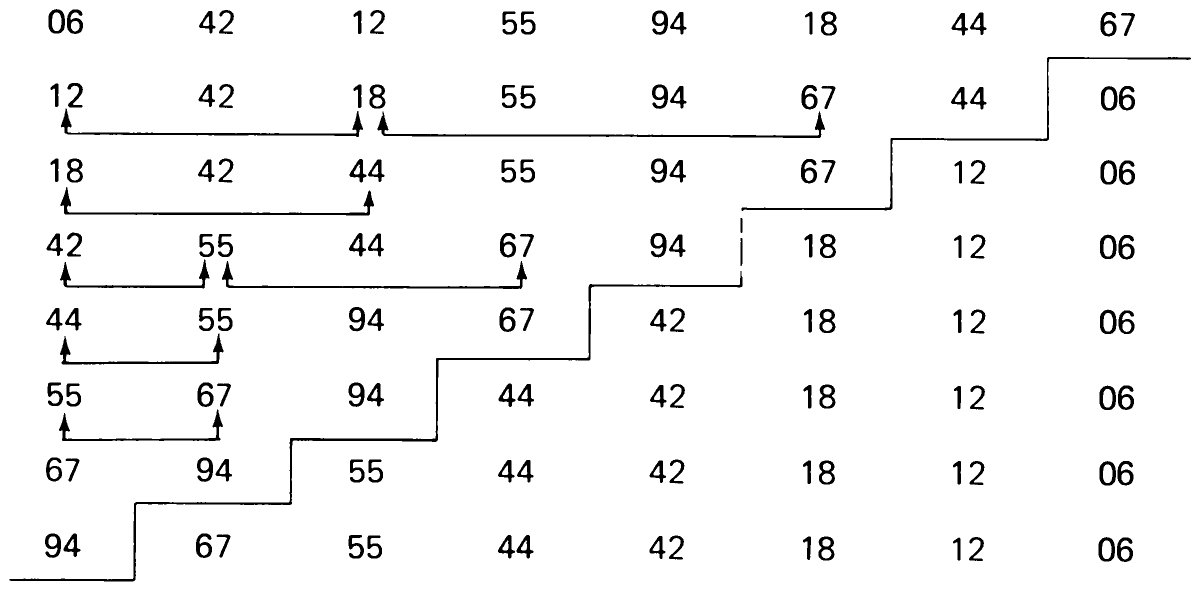
In order to obtain the elements sorted, $n$ sift steps have now to be executed, where after each step the subsequent item may be picked off the top of the heap. Once more, there arise the questions of where to store the emerging top elements and whether or not an in situ sort would be possible. Of course, there is such a solution! In each step take the last component (say $x$) off the heap, store the top element of the heap in the now free location of $x$, and let $x$ sift down into its proper position. The necessary $n - 1$ steps are illustrated on the heap of Table 2.7. The process is described with the aid of the sift75 procedure (Program 2.7) as follows:

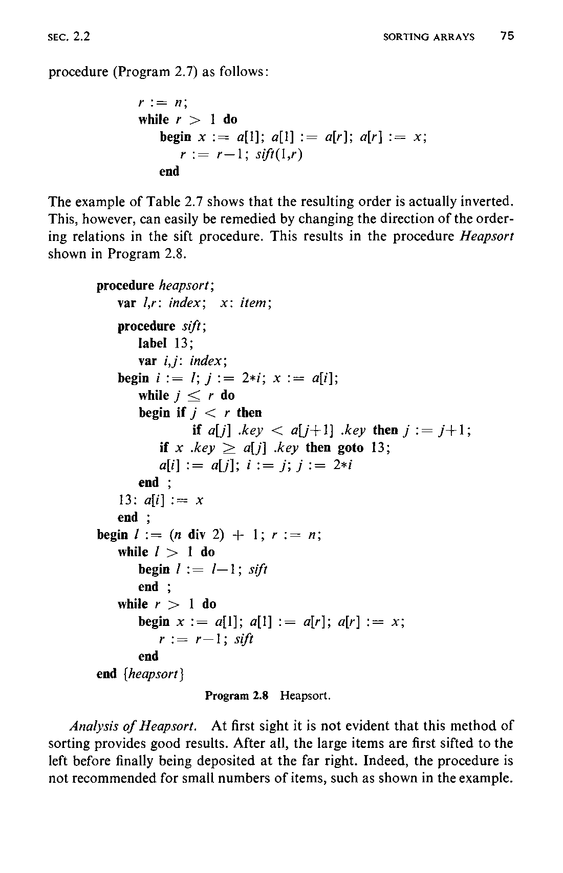
r := n;
while r > 1 do
  begin x := a[1]; a[1] := a[r]; a[r] := x;
    r := r-1; sift(1,r)
  end

The example of Table 2.7 shows that the resulting order is actually inverted. This, however, can easily be remedied by changing the direction of the ordering relations in the sift procedure. This results in the procedure Heapsort shown in Program 2.8.

procedure heapsort;
  var l,r: index;  x: item;

  procedure sift;
    label 13;
    var i,j: index;
  begin i := l; j := 2*i; x := a[i];
    while j ≤ r do
    begin if j < r then
            if a[j] .key < a[j+1] .key then j := j+1;
      if x .key ≥ a[j] .key then goto 13;
      a[i] := a[j]; i := j; j := 2*i
    end ;
  13: a[i] := x
  end ;
begin l := (n div 2) + 1; r := n;
  while l > 1 do
    begin l := l-1; sift
    end ;
  while r > 1 do
    begin x := a[1]; a[1] := a[r]; a[r] := x;
      r := r-1; sift
    end
end {heapsort}

Analysis of Heapsort. At first sight it is not evident that this method of sorting provides good results. After all, the large items are first sifted to the left before finally being deposited at the far right. Indeed, the procedure is not recommended for small numbers of items, such as shown in the example.76 However, for large $n$, Heapsort is very efficient, and the larger the $n$, the better it is—even compared to Shellsort.

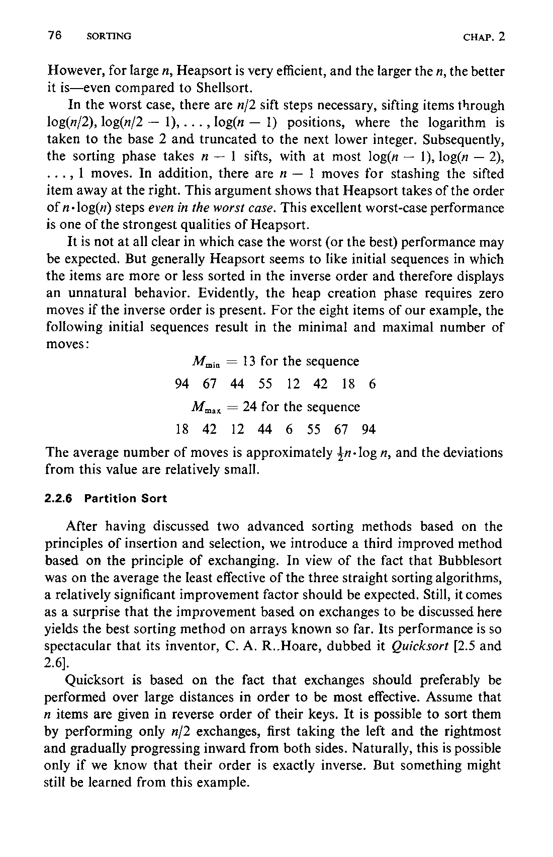
In the worst case, there are $n/2$ sift steps necessary, sifting items through $\log(n/2), \log(n/2 - 1), \dots, \log(n - 1)$ positions, where the logarithm is taken to the base 2 and truncated to the next lower integer. Subsequently, the sorting phase takes $n - 1$ sifts, with at most $\log(n - 1), \log(n - 2), \dots, 1$ moves. In addition, there are $n - 1$ moves for stashing the sifted item away at the right. This argument shows that Heapsort takes of the order of $n \cdot \log(n)$ steps even in the worst case. This excellent worst-case performance is one of the strongest qualities of Heapsort.

It is not at all clear in which case the worst (or the best) performance may be expected. But generally Heapsort seems to like initial sequences in which the items are more or less sorted in the inverse order and therefore displays an unnatural behavior. Evidently, the heap creation phase requires zero moves if the inverse order is present. For the eight items of our example, the following initial sequences result in the minimal and maximal number of moves:

The average number of moves is approximately $\frac{1}{2} n \cdot \log n$, and the deviations from this value are relatively small.

2.2.6 Partition Sort

After having discussed two advanced sorting methods based on the principles of insertion and selection, we introduce a third improved method based on the principle of exchanging. In view of the fact that Bubblesort was on the average the least effective of the three straight sorting algorithms, a relatively significant improvement factor should be expected. Still, it comes as a surprise that the improvement based on exchanges to be discussed here yields the best sorting method on arrays known so far. Its performance is so spectacular that its inventor, C. A. R..Hoare, dubbed it Quicksort [2.5 and 2.6].

Quicksort is based on the fact that exchanges should preferably be performed over large distances in order to be most effective. Assume that $n$ items are given in reverse order of their keys. It is possible to sort them by performing only $n/2$ exchanges, first taking the left and the rightmost and gradually progressing inward from both sides. Naturally, this is possible only if we know that their order is exactly inverse. But something might still be learned from this example.

77 Let us try the following algorithm: Pick any item at random (and call it $x$); scan the array from the left until an item $a_i > x$ is found and then scan from the right until an item $a_j < x$ is found. Now exchange the two items and continue this “scan and swap” process until the two scans meet somewhere in the middle of the array. The result is that the array is now partitioned into a left part with keys less than $x$ and a right part with keys greater than $x$. This partitioning process is now formulated in the form of a procedure in Program 2.9. Note that the relations $>$ and $<$ have been replaced by $\ge$ and $\le$ whose negation in the while clause is $<$ and $>$. With this change $x$ acts as a sentinel for both scans.

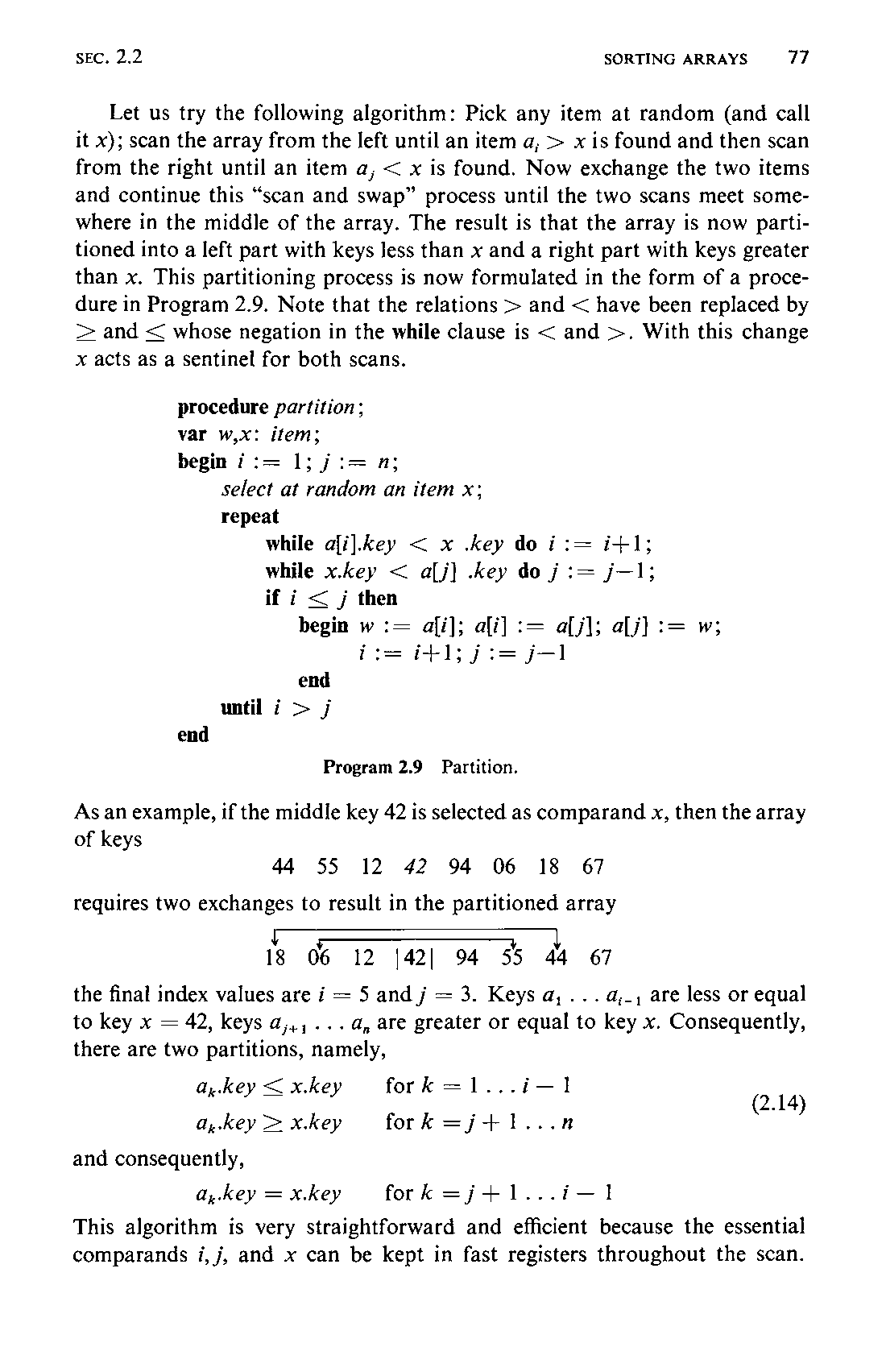
procedure partition;
var w,x: item;
begin i := 1; j := n;
   select at random an item x;
   repeat
      while a[i].key < x .key do i := i+1;
      while x.key < a[j] .key do j := j-1;
      if i ≤ j then
        begin w := a[i]; a[i] := a[j]; a[j] := w;
              i := i+1; j := j-1
        end
   until i > j
end

As an example, if the middle key 42 is selected as comparand $x$, then the array of keys

requires two exchanges to result in the partitioned array

the final index values are $i = 5$ and $j = 3$. Keys $a_1 \dots a_{i-1}$ are less or equal to key $x = 42$, keys $a_{j+1} \dots a_n$ are greater or equal to key $x$. Consequently, there are two partitions, namely,

and consequently,

This algorithm is very straightforward and efficient because the essential comparands $i$, $j$, and $x$ can be kept in fast registers throughout the scan.78 However, it can also be cumbersome, as witnessed by the case with $n$ identical keys, which results in $n/2$ exchanges. These unnecessary exchanges might easily be eliminated by changing the scanning statements to

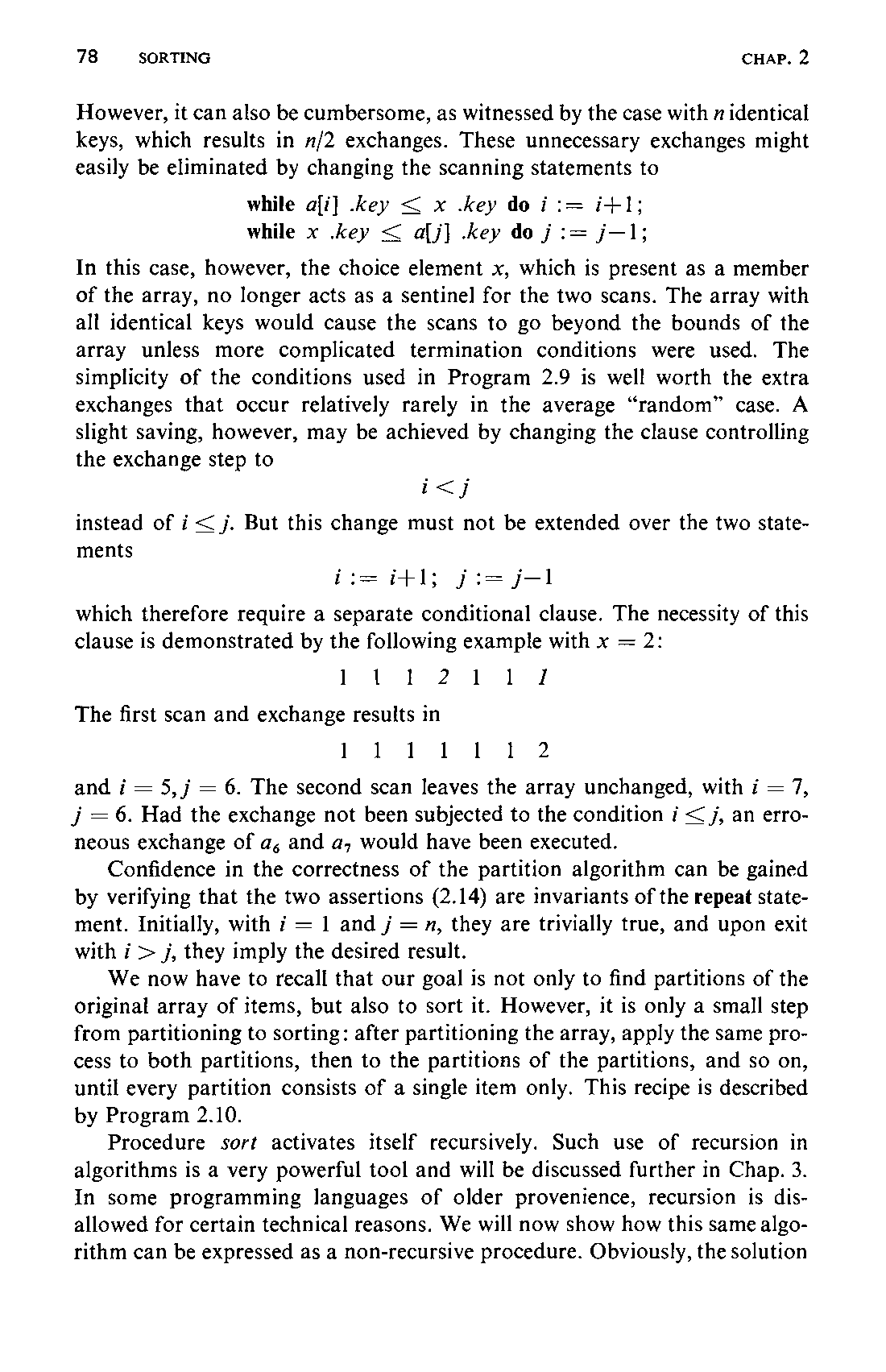
while a[i] .key ≤ x .key do i := i+1;
while x .key ≤ a[j] .key do j := j-1;

In this case, however, the choice element $x$, which is present as a member of the array, no longer acts as a sentinel for the two scans. The array with all identical keys would cause the scans to go beyond the bounds of the array unless more complicated termination conditions were used. The simplicity of the conditions used in Program 2.9 is well worth the extra exchanges that occur relatively rarely in the average “random” case. A slight saving, however, may be achieved by changing the clause controlling the exchange step to

instead of $i \le j$. But this change must not be extended over the two statements

i := i+1;  j := j-1

which therefore require a separate conditional clause. The necessity of this clause is demonstrated by the following example with $x = 2$:

The first scan and exchange results in

and $i = 5$, $j = 6$. The second scan leaves the array unchanged, with $i = 7$, $j = 6$. Had the exchange not been subjected to the condition $i \le j$, an erroneous exchange of $a_6$ and $a_7$ would have been executed.

Confidence in the correctness of the partition algorithm can be gained by verifying that the two assertions (2.14) are invariants of the repeat statement. Initially, with $i = 1$ and $j = n$, they are trivially true, and upon exit with $i > j$, they imply the desired result.

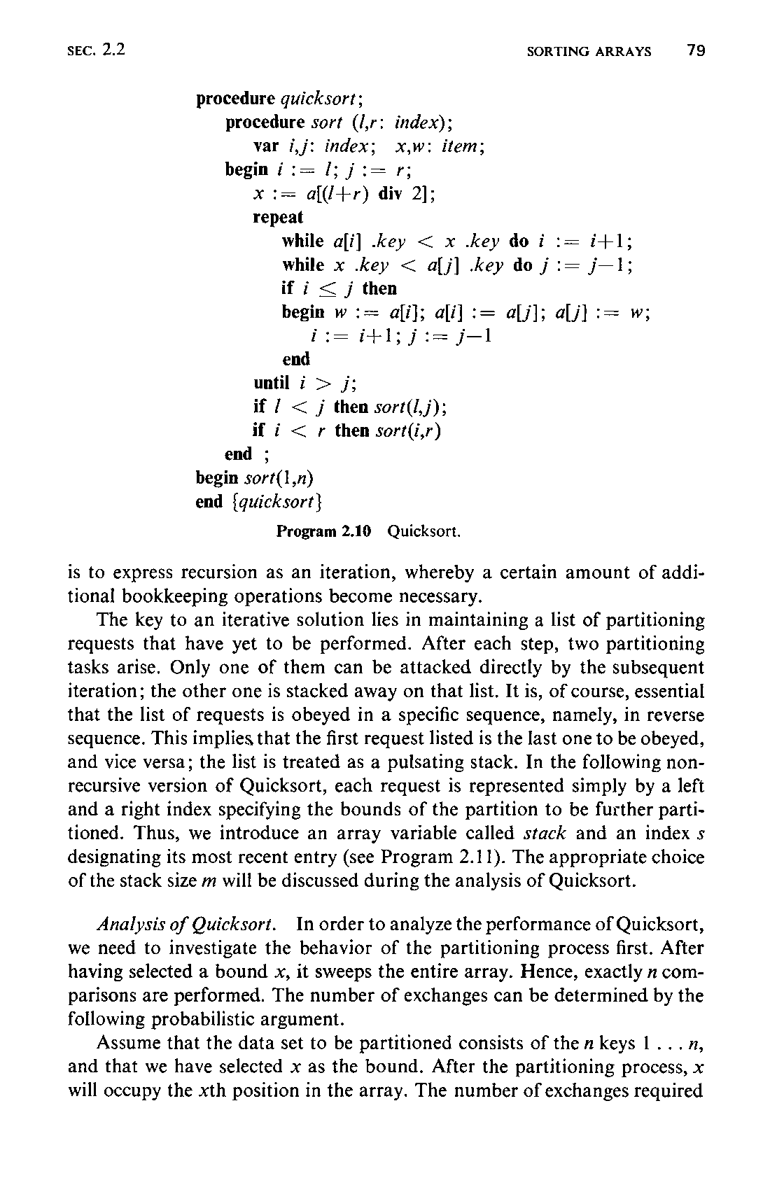
We now have to recall that our goal is not only to find partitions of the original array of items, but also to sort it. However, it is only a small step from partitioning to sorting: after partitioning the array, apply the same process to both partitions, then to the partitions of the partitions, and so on, until every partition consists of a single item only. This recipe is described by Program 2.10.

Procedure sort activates itself recursively. Such use of recursion in algorithms is a very powerful tool and will be discussed further in Chap. 3. In some programming languages of older provenience, recursion is disallowed for certain technical reasons. We will now show how this same algorithm can be expressed as a non-recursive procedure. Obviously, the solution79 is to express recursion as an iteration, whereby a certain amount of additional bookkeeping operations become necessary.

procedure quicksort;
  procedure sort (l,r: index);
    var i,j: index;  x,w: item;
  begin i := l; j := r;
    x := a[(l+r) div 2];
    repeat
      while a[i] .key < x .key do i := i+1;
      while x .key < a[j] .key do j := j-1;
      if i ≤ j then
      begin w := a[i]; a[i] := a[j]; a[j] := w;
        i := i+1; j := j-1
      end
    until i > j;
    if l < j then sort(l,j);
    if i < r then sort(i,r)
  end ;
begin sort(1,n)
end {quicksort}

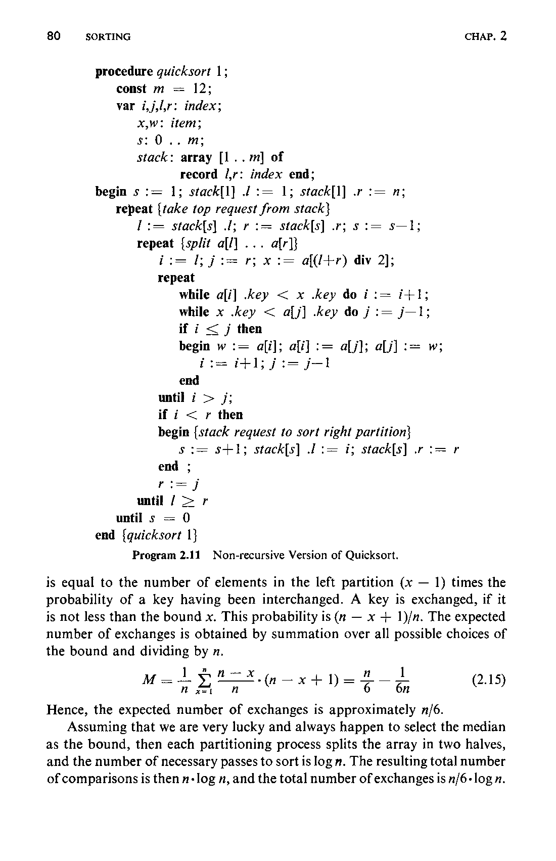
The key to an iterative solution lies in maintaining a list of partitioning requests that have yet to be performed. After each step, two partitioning tasks arise. Only one of them can be attacked directly by the subsequent iteration; the other one is stacked away on that list. It is, of course, essential that the list of requests is obeyed in a specific sequence, namely, in reverse sequence. This implies that the first request listed is the last one to be obeyed, and vice versa; the list is treated as a pulsating stack. In the following non-recursive version of Quicksort, each request is represented simply by a left and a right index specifying the bounds of the partition to be further partitioned. Thus, we introduce an array variable called stack and an index $s$ designating its most recent entry (see Program 2.11). The appropriate choice of the stack size $m$ will be discussed during the analysis of Quicksort.

Analysis of Quicksort. In order to analyze the performance of Quicksort, we need to investigate the behavior of the partitioning process first. After having selected a bound $x$, it sweeps the entire array. Hence, exactly $n$ comparisons are performed. The number of exchanges can be determined by the following probabilistic argument.

Assume that the data set to be partitioned consists of the $n$ keys $1 \dots n$, and that we have selected $x$ as the bound. After the partitioning process, $x$ will occupy the $x$th position in the array. The number of exchanges required80 is equal to the number of elements in the left partition $(x - 1)$ times the probability of a key having been interchanged. A key is exchanged, if it is not less than the bound $x$. This probability is $(n - x + 1)/n$. The expected number of exchanges is obtained by summation over all possible choices of the bound and dividing by $n$.

procedure quicksort 1;
  const m = 12;
  var i,j,l,r: index;
    x,w: item;
    s: 0 .. m;
    stack: array [1 .. m] of
             record l,r: index end;
begin s := 1; stack[1] .l := 1; stack[1] .r := n;
  repeat {take top request from stack}
    l := stack[s] .l; r := stack[s] .r; s := s-1;
    repeat {split a[l] ... a[r]}
      i := l; j := r; x := a[(l+r) div 2];
      repeat
        while a[i] .key < x .key do i := i+1;
        while x .key < a[j] .key do j := j-1;
        if i ≤ j then
        begin w := a[i]; a[i] := a[j]; a[j] := w;
          i := i+1; j := j-1
        end
      until i > j;
      if i < r then
      begin {stack request to sort right partition}
        s := s+1; stack[s] .l := i; stack[s] .r := r
      end ;
      r := j
    until l ≥ r
  until s = 0
end {quicksort 1}

Hence, the expected number of exchanges is approximately $n/6$.

Assuming that we are very lucky and always happen to select the median as the bound, then each partitioning process splits the array in two halves, and the number of necessary passes to sort is $\log n$. The resulting total number of comparisons is then $n \cdot \log n$, and the total number of exchanges is $n/6 \cdot \log n$.

81 Of course, one cannot expect to hit the median all the time. In fact, the chance of doing so is only $1/n$. Surprisingly, however, the average performance of Quicksort is inferior to the optimal case by a factor of only $2 \cdot \ln 2$ if the bound is chosen at random.

But Quicksort does have its pitfalls. First of all, it performs moderately well for small values of $n$, as do all advanced methods. Its advantage over the other advanced methods lies in the ease with which a straight sorting method can be incorporated to handle small partitions. This is particularly advantageous when considering the recursive version of the program.

Still, there remains the question of the worst case. How does Quicksort perform then? The answer is unfortunately disappointing and it unveils the one weakness of Quicksort (which in those cases becomes Slowsort). Consider, for instance, the unlucky case in which each time the largest value of a partition happens to be picked as comparand $x$. Then each step splits a segment of $n$ items into a left partition with $n - 1$ and a right partition with one single item. The result is that $n$ instead of only $\log n$ splits become necessary and that the worst-case performance is of the order $n^2$.

Apparently, the crucial step is the selection of the comparand $x$. In our example program it is chosen as the middle element. Note that one might almost as well select either the first or the last element a[l] or a[r]. In these cases, the worst case is the initially sorted array; Quicksort then shows a definite dislike for the trivial job and a preference for disordered arrays. In choosing the middle element, the strange characteristic of Quicksort is less obvious because the initially sorted array becomes the optimal case! In fact, the average performance is slightly better if the middle element is selected. Hoare suggests that the choice of $x$ be made “at random” or by selecting it as the median of a small sample of, say, three keys [2.12 and 2.13]. Such a judicious choice hardly influences the average performance of Quicksort, but it improves the worst-case performance considerably. It becomes evident that sorting on the basis of Quicksort is somewhat like a gamble in which one should be aware of how much one may afford to lose if bad luck were to strike.

There is one important lesson to be learned from this experience; it concerns the programmer directly. What are the consequences of the worst case behavior mentioned above to the performance of Program 2.11? We have realized that each split results in a right partition of only a single element; the request to sort this partition is stacked for later execution. Consequently, the maximum number of requests, and therefore the total required stack size, is $n$. This is, of course, totally unacceptable. (Note that we fare no better—and, in fact, even worse—with the recursive version because a system allowing recursive activation of procedures will have to store the values of local variables and parameters of all procedure activations82 automatically, and it will use an implicit stack for this purpose.) The remedy lies in stacking the sort request for the longer partition and in continuing directly with the further partitioning of the smaller sections. In this case, the size of the stack $m$ can be limited to $m = \log_2 n$.

The change necessary to Program 2.11 is localized in the section setting up new requests. It now reads

if j-l < r-i then
begin if i < r then
    begin {stack request for sorting right partition}
       s := s+1; stack[s] .l := i; stack[s] .r := r
    end;
    r := j  {continue sorting left partition}
end else
begin if l < j then
    begin {stack request for sorting left partition}
       s := s+1; stack[s] .l := l; stack[s] .r := j
    end;
    l := i  {continue sorting right partition}
end

2.2.7 Finding the Median

The median of $n$ items is defined as that item which is less than (or equal to) half of the $n$ items and which is larger than (or equal to) the other half of the $n$ items. For example, the median of

is 18.

The problem of finding the median is customarily connected with that of sorting because one sure method of determining the median is to sort the $n$ items and then to pick the item in the middle. But partitioning by Program 2.9 yields a potentially much faster way of finding the median. The method to be displayed easily generalizes to the problem of finding the $k$th smallest of $n$ items. Finding the median represents the special case $k = n/2$.

The algorithm invented by C. A. R. Hoare [2-4] functions as follows. First, the partitioning operation of Quicksort is applied with $l = 1$ and $r = n$ and with a[k] selected as splitting value (bound) $x$. The resulting index values $i$ and $j$ are such that

83 There are three possible cases that may arise:

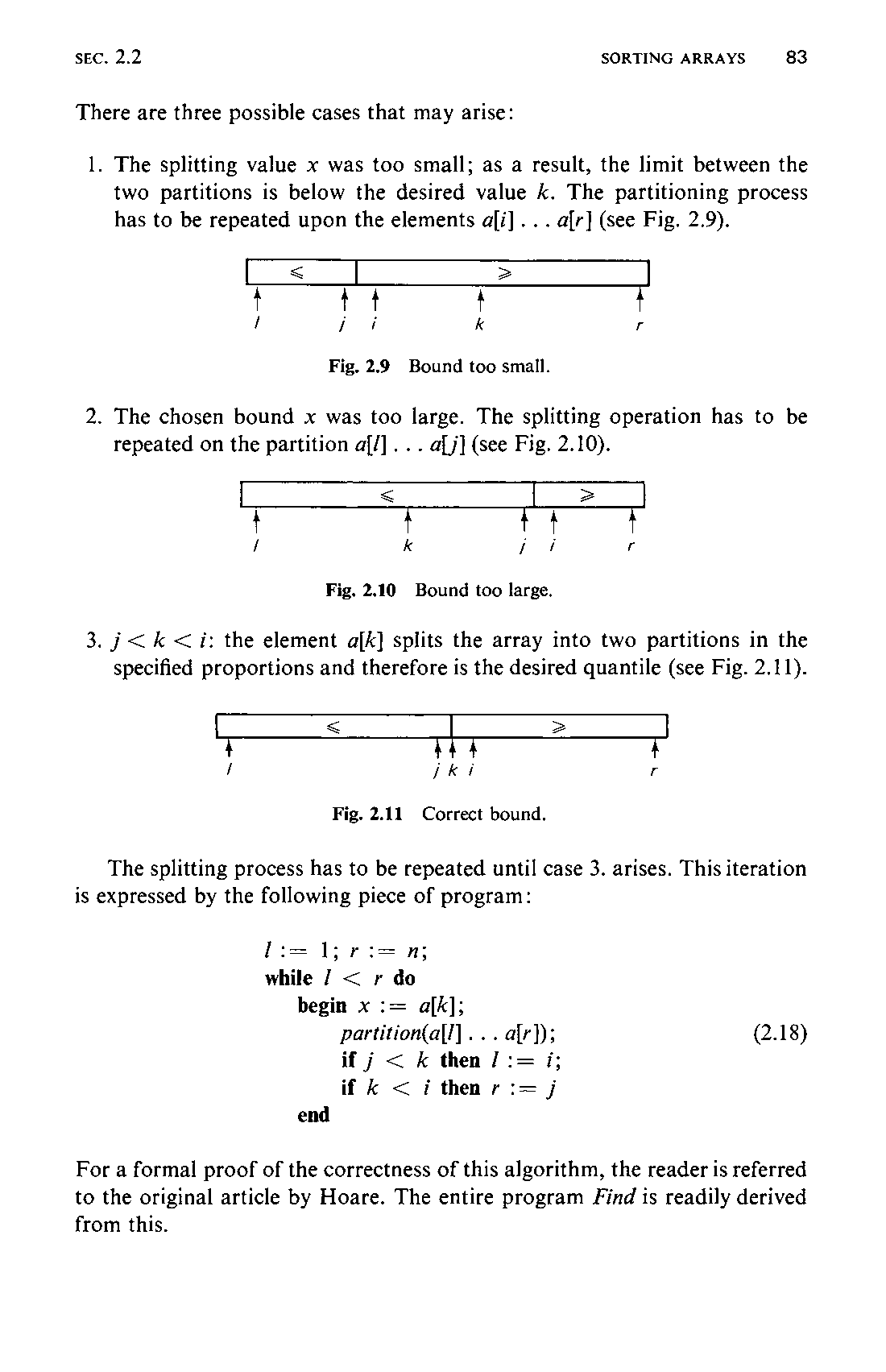
1. The splitting value $x$ was too small; as a result, the limit between the two partitions is below the desired value $k$. The partitioning process has to be repeated upon the elements a[i] … a[r] (see Fig. 2.9).

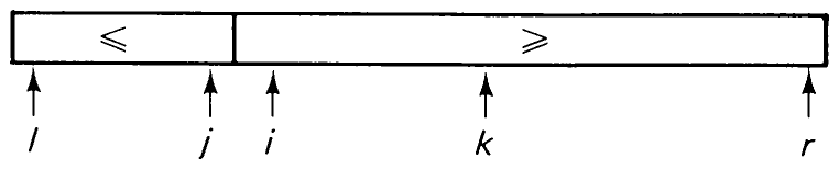
2. The chosen bound $x$ was too large. The splitting operation has to be repeated on the partition a[l] … a[j] (see Fig. 2.10).

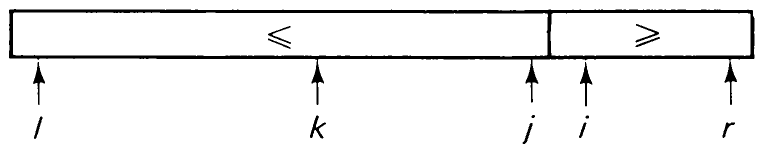
3. $j < k < i$: the element a[k] splits the array into two partitions in the specified proportions and therefore is the desired quantile (see Fig. 2.11).

The splitting process has to be repeated until case 3. arises. This iteration is expressed by the following piece of program:

l := 1; r := n;
while l < r do
  begin x := a[k];
        partition(a[l] ... a[r]);
        if j < k then l := i;
        if k < i then r := j
  end

For a formal proof of the correctness of this algorithm, the reader is referred to the original article by Hoare. The entire program Find is readily derived from this.

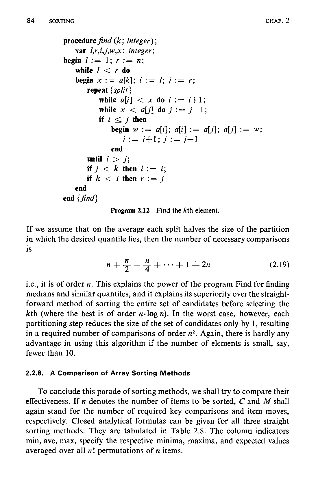
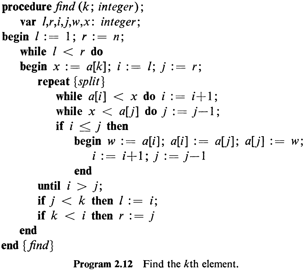
If we assume that on the average each split halves the size of the partition in which the desired quantile lies, then the number of necessary comparisons is

i.e., it is of order n. This explains the power of the program Find for finding medians and similar quantiles, and it explains its superiority cover the straightforward method of sorting the entire set of candidates before selecting the kth (where the best is of order n-log n). In the worst case, however, each partitioning step reduces the size of the set of candidates only by 1, resulting in a required number of comparisons of order n?. Again, there is hardly any advantage in using this algorithm if the number of elements is small, say, fewer than 10.

2.2.8 A Comparison of Array Sorting Methods

To conclude this parade of sorting methods, we shall try to compare their effectiveness. If n denotes the number of items to be sorted, C and M shall again stand for the number of required key comparisons and item moves, respectively. Closed analytical formulas can be given for all three straight sorting methods. They are tabulated in Table 2.8. The column indicators min, ave, max, specify the respective minima, maxima, and expected values averaged over all m! permutations of n items.

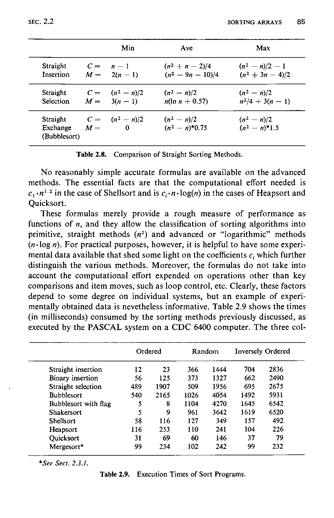
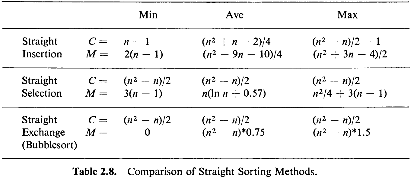
No reasonably simple accurate formulas are available on the advanced methods. The essential facts are that the computational effort needed is c,-n'-? in the case of Shellsort and is c,-n-log() in the cases of Heapsort and Quicksort.

These formulas merely provide a rough measure of performance as functions of n, and they allow the classification of sorting algorithms into primitive, straight methods (m?) and advanced or “logarithmic” methods (n-log n). For practical purposes, however, it is helpful to have some experimental data available that shed some light on the coefficients c, which further distinguish the various methods. Moreover, the formulas do not take into account the computational effort expended on operations other than key comparisons and item moves, such as loop control, etc. Clearly, these factors depend to some degree on individual systems, but an example of experimentally obtained data is nevetheless informative. Table 2.9 shows the times (in milliseconds) consumed by the sorting methods previously discussed, as executed by the PASCAL system on a CDC 6400 computer. The three col-

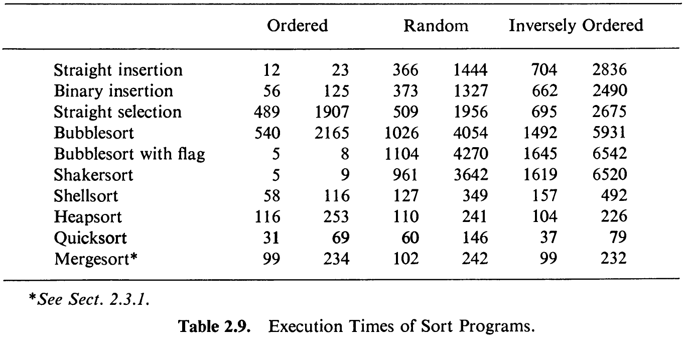
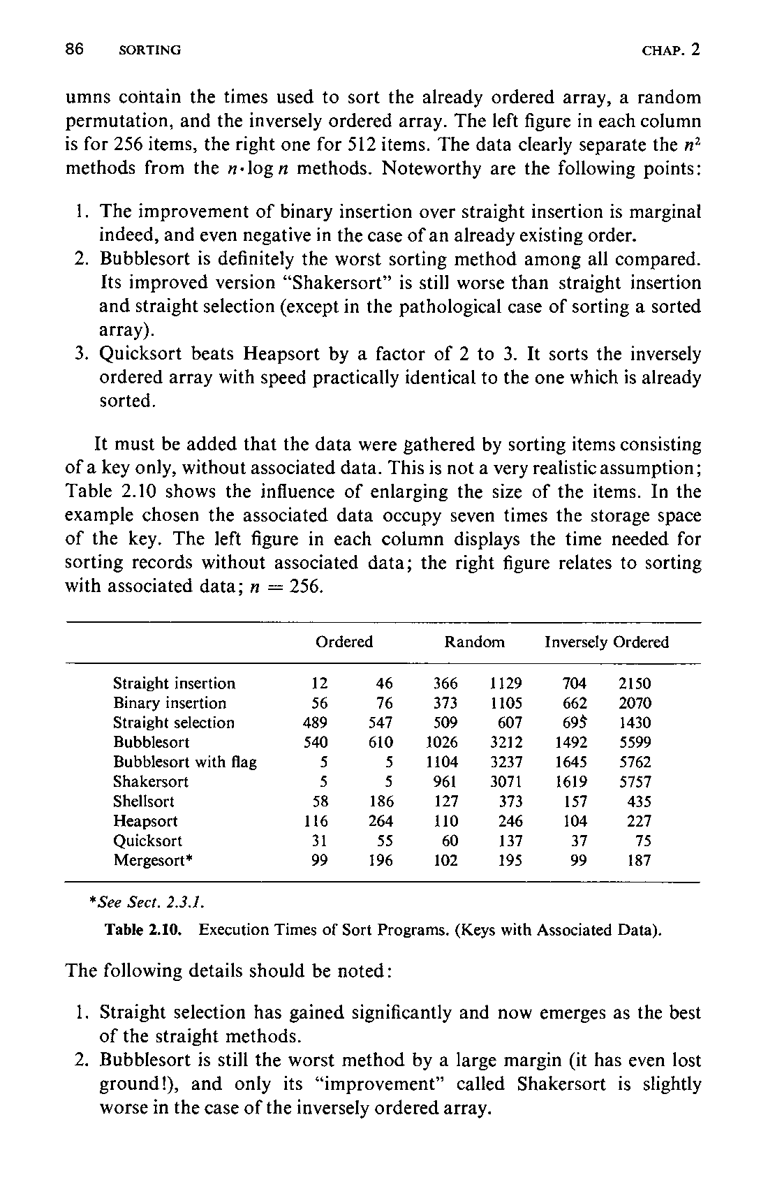
umns contain the times used to sort the already ordered array, a random permutation, and the inversely ordered array. The left figure in each column is for 256 items, the right one for 512 items. The data clearly separate the n? methods from the n-logn methods. Noteworthy are the following points:

1. The improvement of binary insertion over straight insertion is marginal indeed, and even negative in the case of an already existing order.

2. Bubblesort is definitely the worst sorting method among all compared. Its improved version “Shakersort” is still worse than straight insertion and straight selection (except in the pathological case of sorting a sorted array).

3. Quicksort beats Heapsort by a factor of 2 to 3. It sorts the inversely ordered array with speed practically identical to the one which is already sorted.

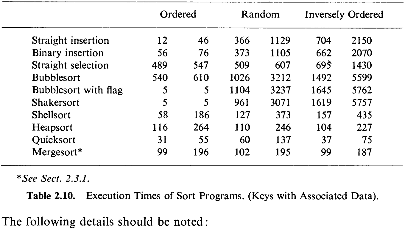
It must be added that the data were gathered by sorting items consisting of a key only, without associated data. This is not a very realistic assumption; Table 2.10 shows the influence of enlarging the size of the items. In the example chosen the associated data occupy seven times the storage space of the key. The left figure in each column displays the time needed for sorting records without associated data; the right figure relates to sorting with associated data; n = 256.

1. Straight selection has gained significantly and now emerges as the best of the straight methods.

2. Bubblesort is still the worst method by a large margin (it has even lost ground!), and only its “improvement” called Shakersort is slightly worse in the case of the inversely ordered array.

3. Quicksort has even strengthened its position as the quickest method and appears as the best array sorter by far.