Two Examples of Recursive Programs

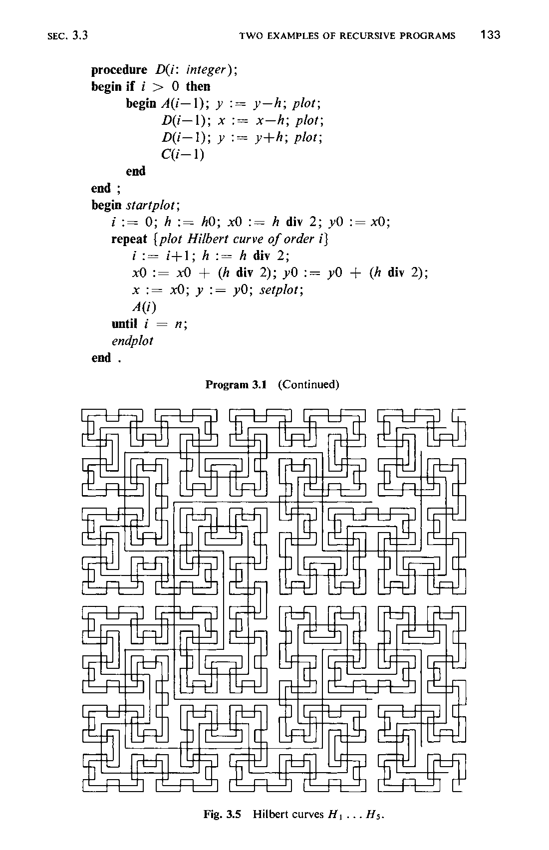
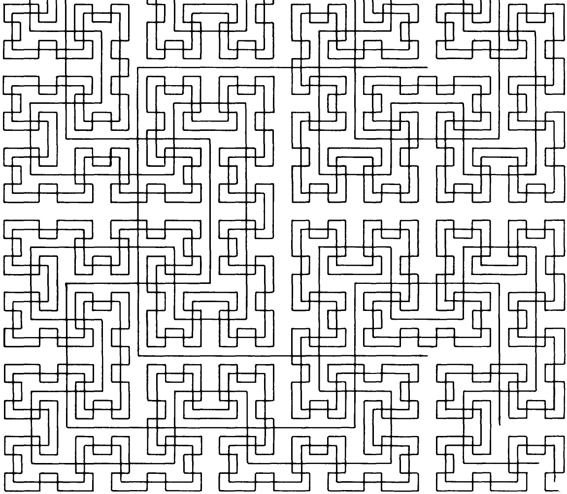
The attractive graphic pattern shown in Fig. 3.5 consists of the superposition of five curves. These curves follow a regular pattern and suggest that they might be drawn by a plotter under control of a computer. Our goal is to discover the recursion schema, according to which the plotting program might be constructed. Inspection reveals that three of the superimposed curves have the shapes shown in Fig. 3.3; we denote them by HA, H,, and H,. The figures show that H,.., is obtained by the composition of four instances of H, of half size and appropriate rotation and by tying together

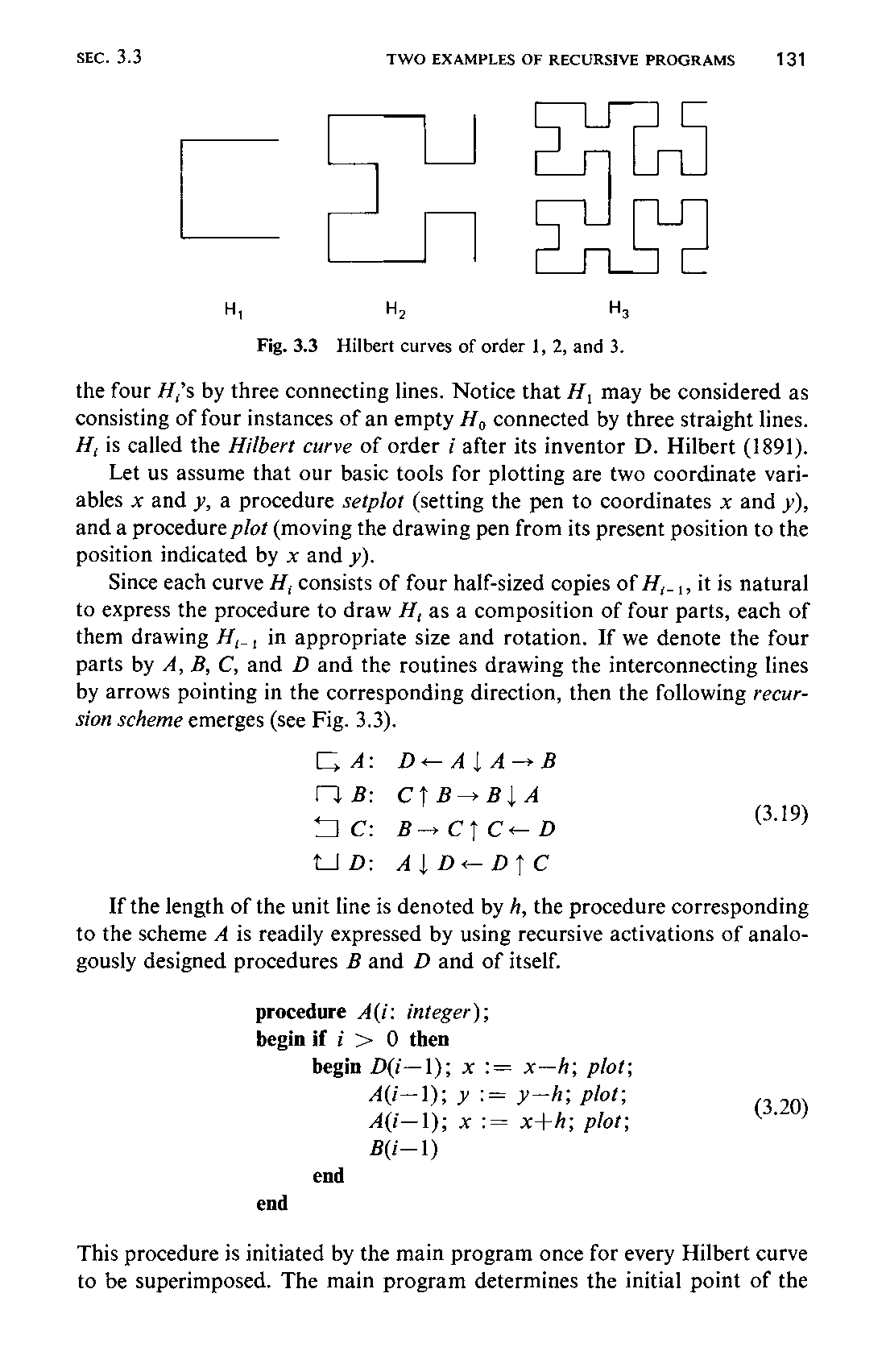
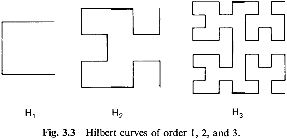
the four H,’s by three connecting lines. Notice that H, may be considered as consisting of four instances of an empty H, connected by three straight lines. H, is called the Hilbert curve of order i after its inventor D. Hilbert (1891).

Let us assume that our basic tools for plotting are two coordinate variables x and y, a procedure setplot (setting the pen to coordinates x and y), and a procedure plot (moving the drawing pen from its present position to the position indicated by x and y).

Since each curve H, consists of four half-sized copies of H,_,, it is natural to express the procedure to draw H, as a composition of four parts, each of them drawing H;_, in appropriate size and rotation. If we denote the four parts by A, B, C, and D and the routines drawing the interconnecting lines by arrows pointing in the corresponding direction, then the following recursion scheme emerges (see Fig. 3.3).

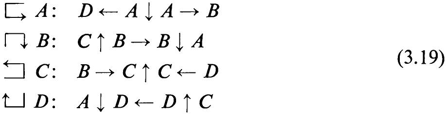
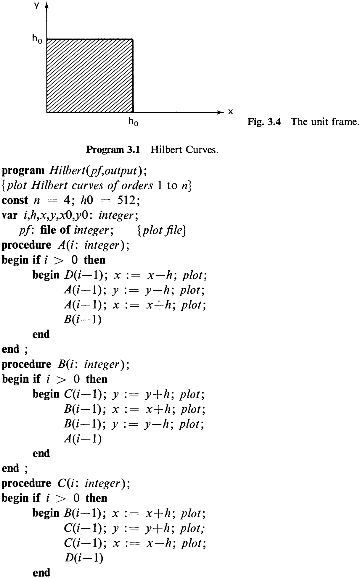
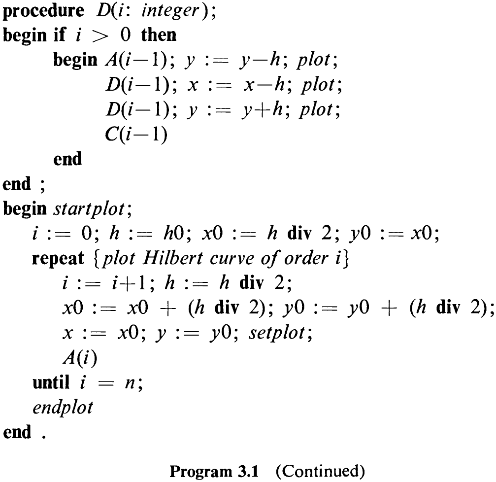
If the length of the unit line is denoted by A, the procedure corresponding to the scheme A is readily expressed by using recursive activations of analogously designed procedures B and D and of itself.

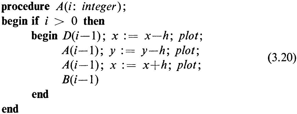
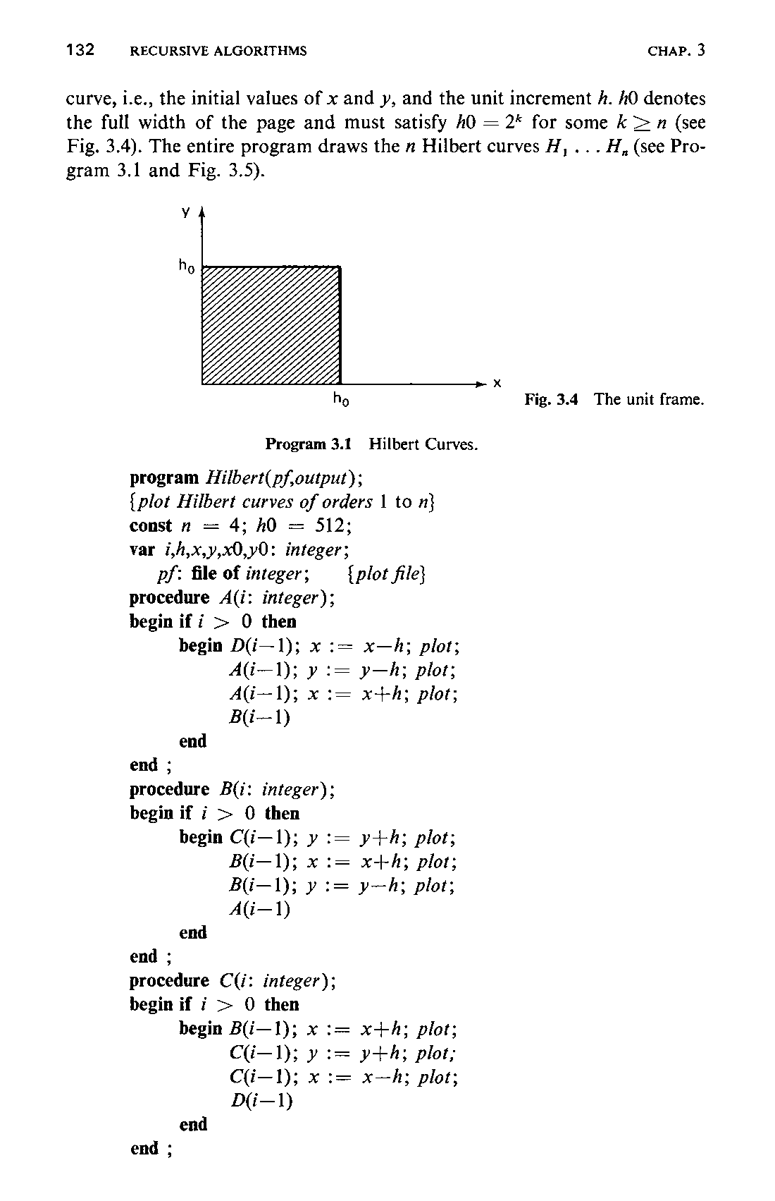
This procedure is initiated by the main program once for every Hilbert curve to be superimposed. The main program determines the initial point of the132 curve, i.e., the initial values of x and y, and the unit increment A. hO denotes the full width of the page and must satisfy 40 = 2* for some k > n (see Fig. 3.4). The entire program draws the n Hilbert curves H, ...H,, (see Program 3.1 and Fig. 3.5).

ttt aS Gates be tal

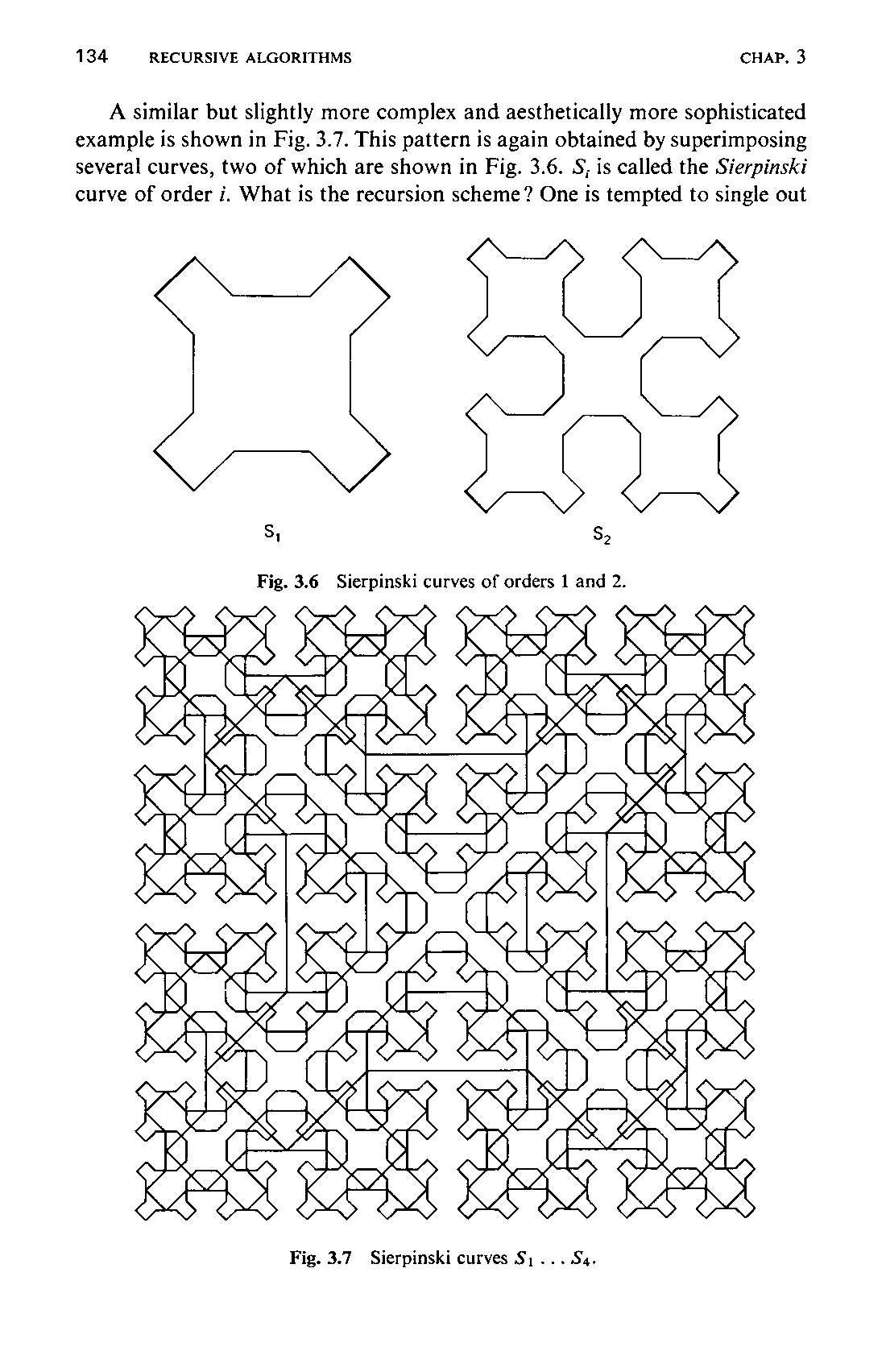
A similar but slightly more complex and aesthetically more sophisticated example is shown in Fig. 3.7. This pattern is again obtained by superimposing several curves, two of which are shown in Fig. 3.6. S; is called the Sierpinski curve of order i. What is the recursion scheme? One is tempted to single out

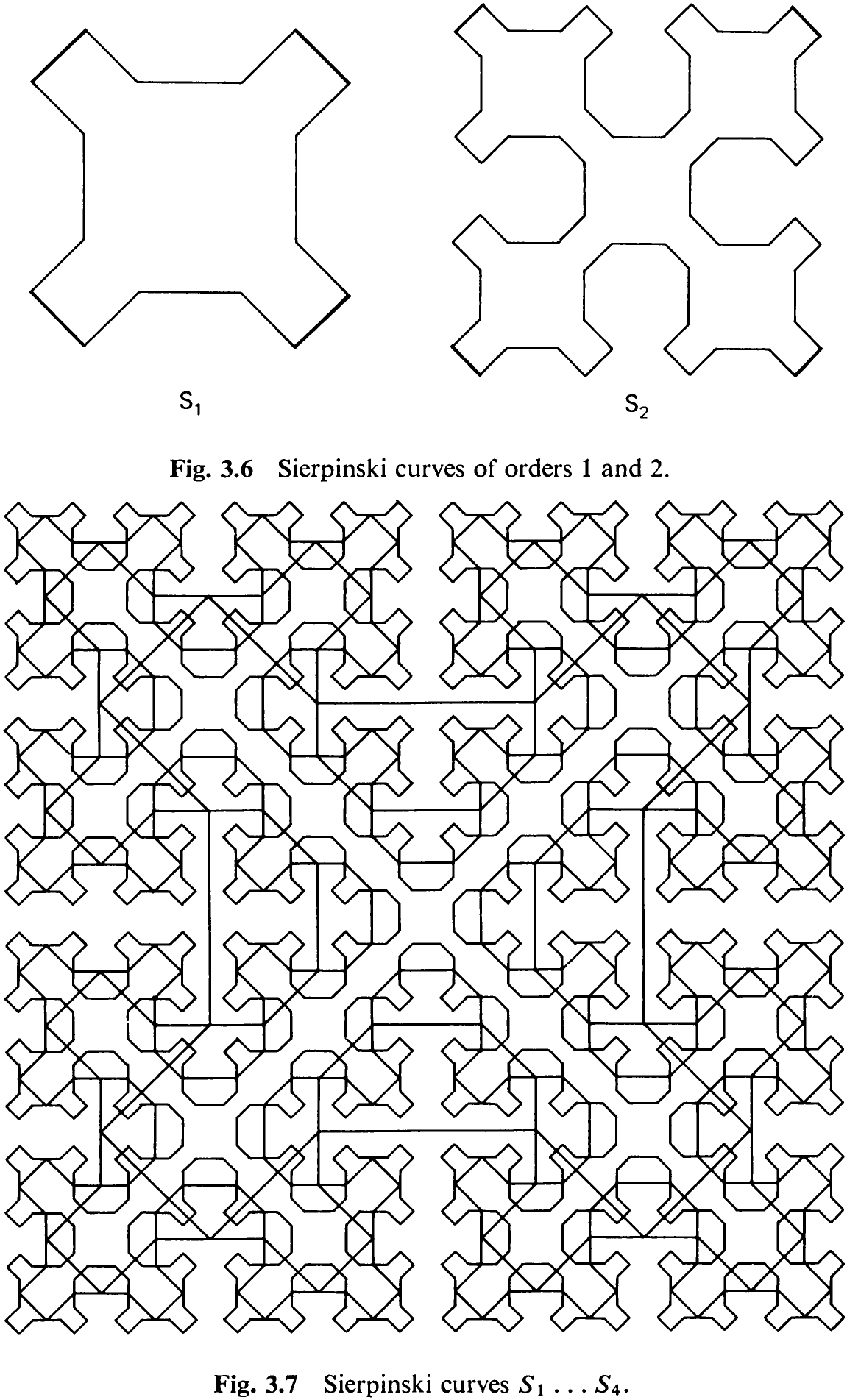
the leaf S, as a basic building block, possibly with one edge left off. But this does not lead to a solution. The principal difference between Sierpinski curves and Hilbert curves is that Sierpinski curves are closed (without crossovers). This implies that the basic recursion scheme must be an open curve and that the four parts are connected by links not belonging to the recursion pattern itself. Indeed, these links consist of the four straight lines in the outermost four “corners,” drawn in boldface in Fig. 3.6. They may be regarded as belonging to a non-empty initial curve S,, which is a square standing on one corner.

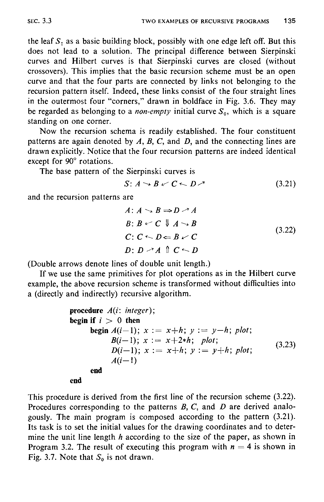
Now the recursion schema is readily established. The four constituent patterns are again denoted by A, B, C, and D, and the connecting lines are drawn explicitly. Notice that the four recursion patterns are indeed identical except for 90° rotations.

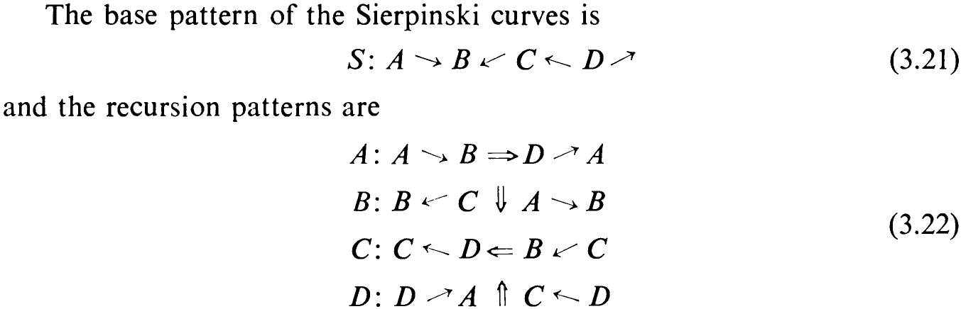
(Double arrows denote lines of double unit length.)

If we use the same primitives for plot operations as in the Hilbert curve example, the above recursion scheme is transformed without difficulties into a (directly and indirectly) recursive algorithm.

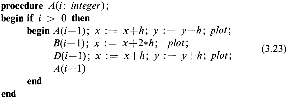
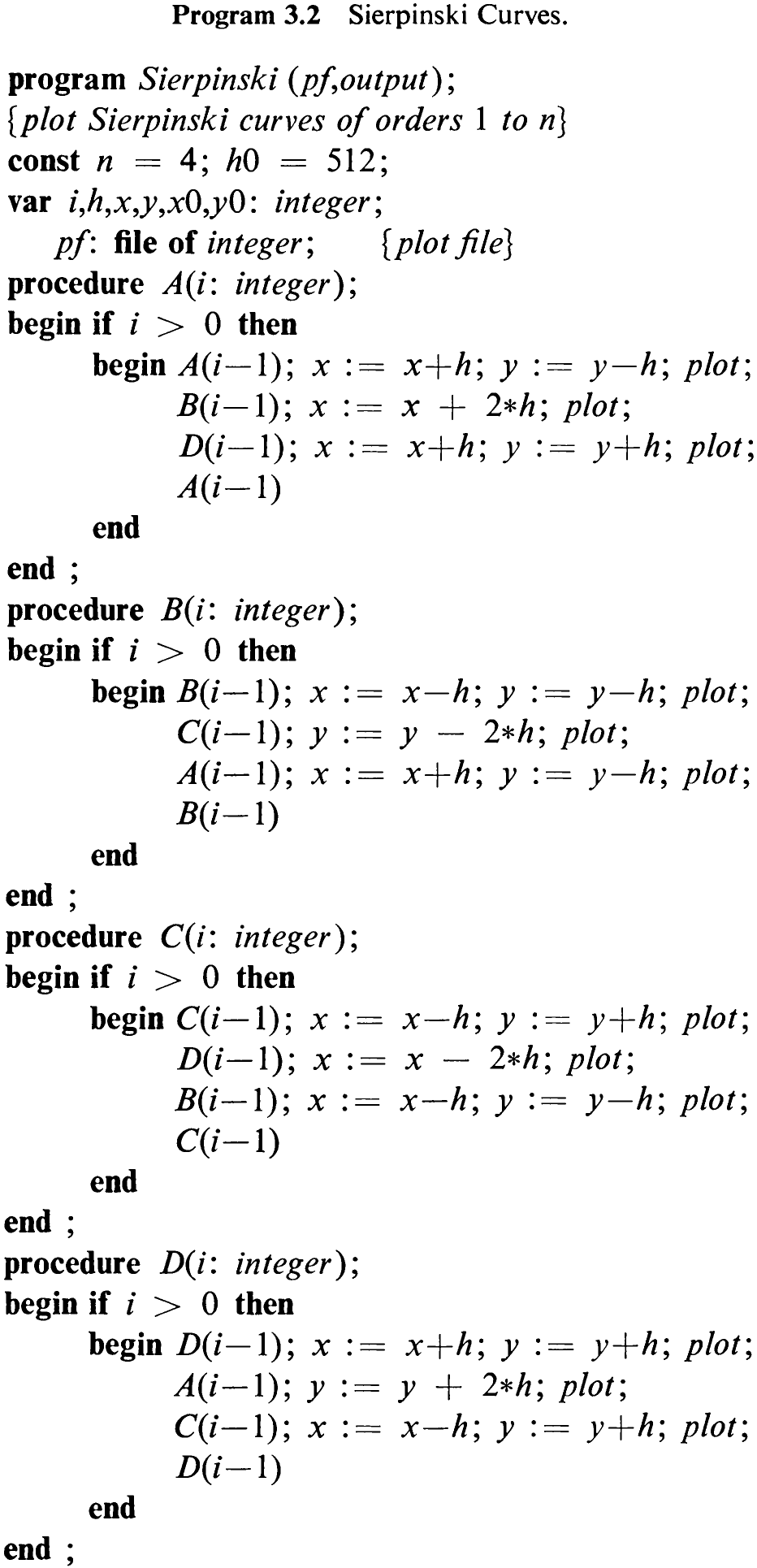
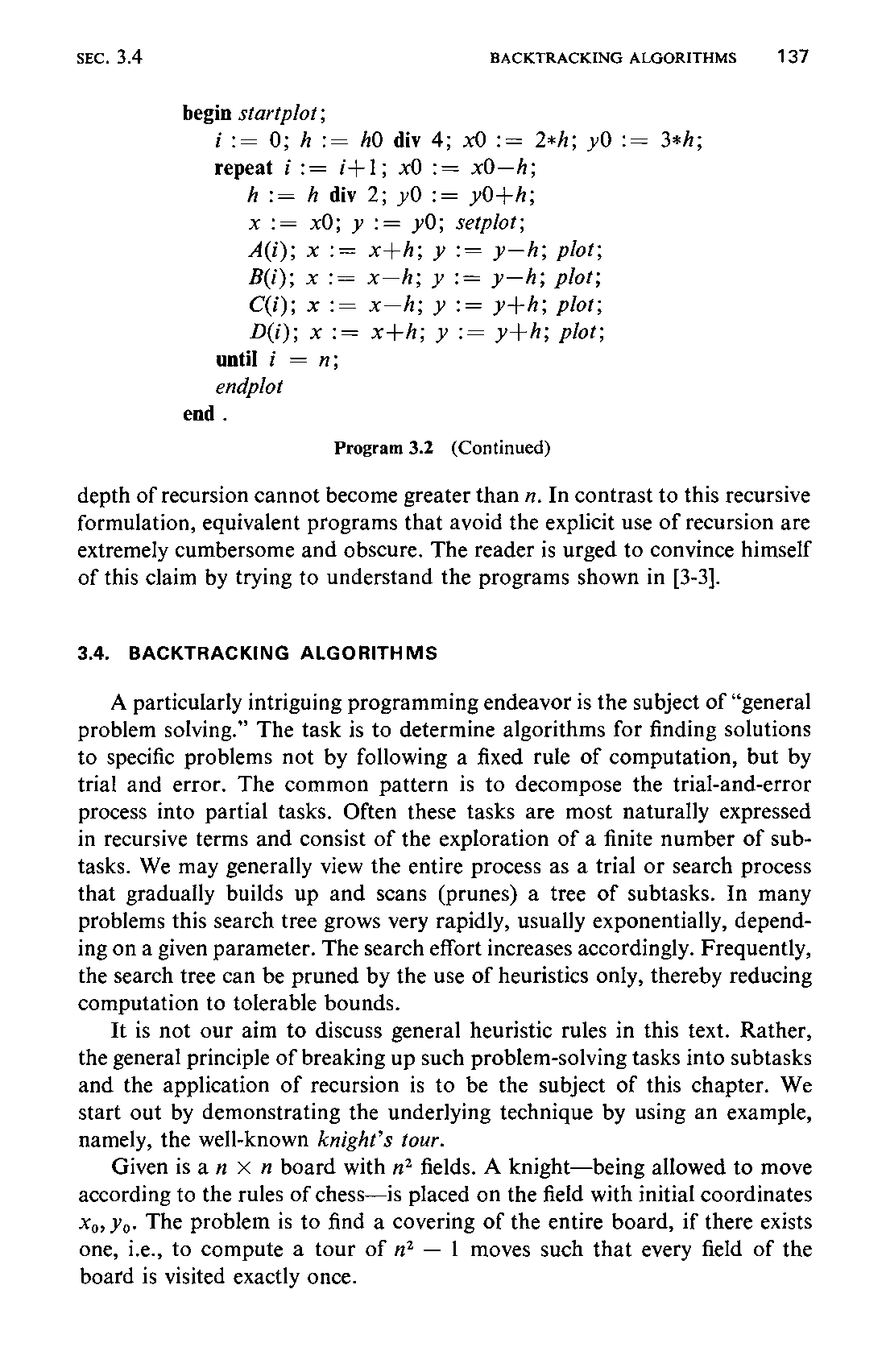
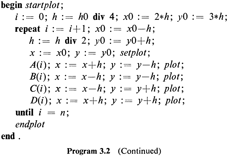
This procedure is derived from the first line of the recursion scheme (3.22). Procedures corresponding to the patterns B, C, and D are derived analogously. The main program is composed according to the pattern (3.21). Its task is to set the initial values for the drawing coordinates and to determine the unit line length # according to the size of the paper, as shown in Program 3.2. The result of executing this program with n = 4 is shown in Fig. 3.7. Note that Sy is not drawn.

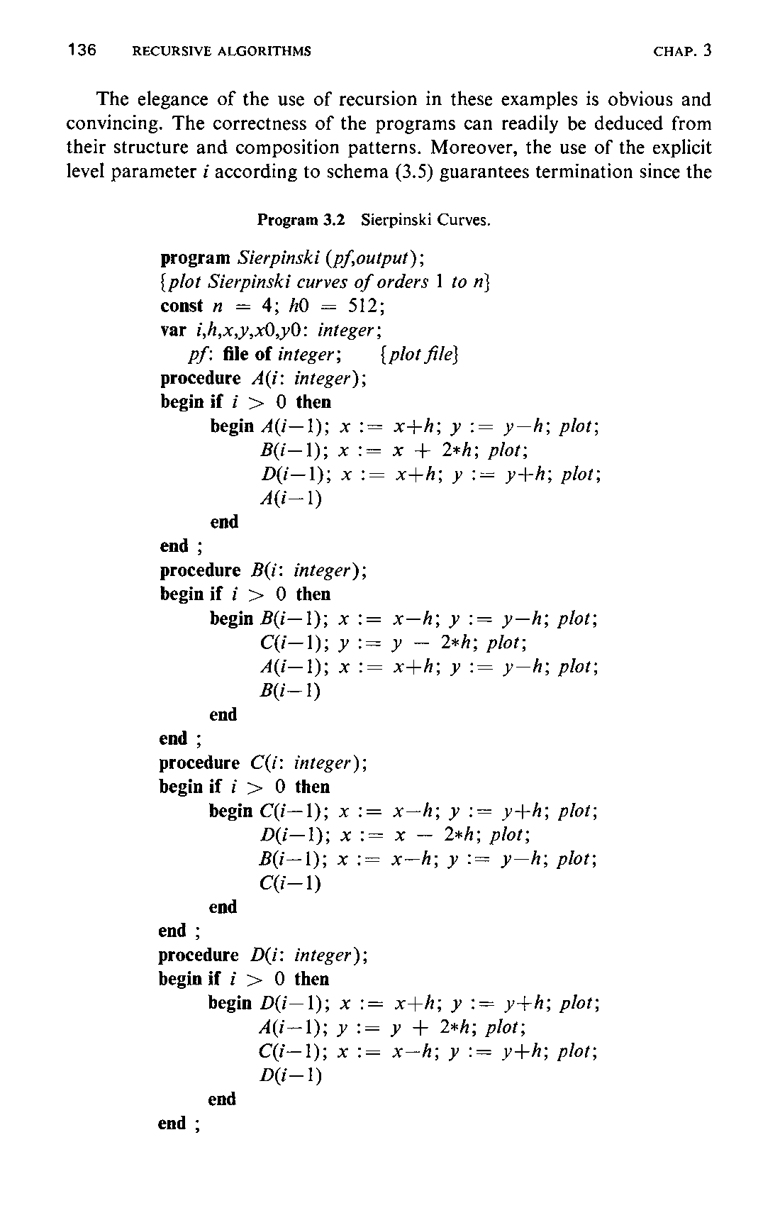
The elegance of the use of recursion in these examples is obvious and convincing. The correctness of the programs can readily be deduced from their structure and composition patterns. Moreover, the use of the explicit level parameter i according to schema (3.5) guarantees termination since the

depth of recursion cannot become greater than x. In contrast to this recursive formulation, equivalent programs that avoid the explicit use of recursion are extremely cumbersome and obscure. The reader is urged to convince himself of this claim by trying to understand the programs shown in [3-3].