Backtracking Algorithms

A particularly intriguing programming endeavor is the subject of “general problem solving.” The task is to determine algorithms for finding solutions to specific problems not by following a fixed rule of computation, but by trial and error. The common pattern is to decompose the trial-and-error process into partial tasks. Often these tasks are most naturally expressed in recursive terms and consist of the exploration of a finite number of subtasks. We may generally view the entire process as a trial or search process that gradually builds up and scans (prunes) a tree of subtasks. In many problems this search tree grows very rapidly, usually exponentially, depending on a given parameter. The search effort increases accordingly. Frequently, the search tree can be pruned by the use of heuristics only, thereby reducing computation to tolerable bounds.

It is not our aim to discuss general heuristic rules in this text. Rather, the general principle of breaking up such problem-solving tasks into subtasks and the application of recursion is to be the subject of this chapter. We start out by demonstrating the underlying technique by using an example, namely, the well-known knight’s tour.

Given is an X n board with n? fields. A knight—being allowed to move according to the rules of chess—is placed on the field with initial coordinates Xo, Yo. The problem is to find a covering of the entire board, if there exists one, i.e., to compute a tour of n? — 1 moves such that every field of the board is visited exactly once.

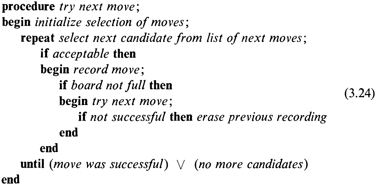
The obvious way to reduce the problem of covering n? fields is to consider the problem of either performing a next move or finding out that none is possible. Let us therefore define an algorithm trying to perform a next move. A first approach is shown in (3.24).

If we wish to be more precise in describing this algorithm, we are forced to make some decisions on data representation. An obvious step is to represent the board by a matrix, say 4. Let us also introduce a type to denote index values:

The decision to represent each field of the board by an integer instead of a Boolean value denoting occupation is because we wish to keep track of the history of successive board occupations. The following convention is an obvious choice:

The next decision concerns the choice of appropriate parameters. They are to determine the starting conditions for the next move and also to report on its success. The former task is adequately solved by specifying the coordinates x, y from which the move is to be made and by specifying the number i of the move (for recording purposes). The latter task requires a Boolean result parameter: g = true denotes success; g = false failure.

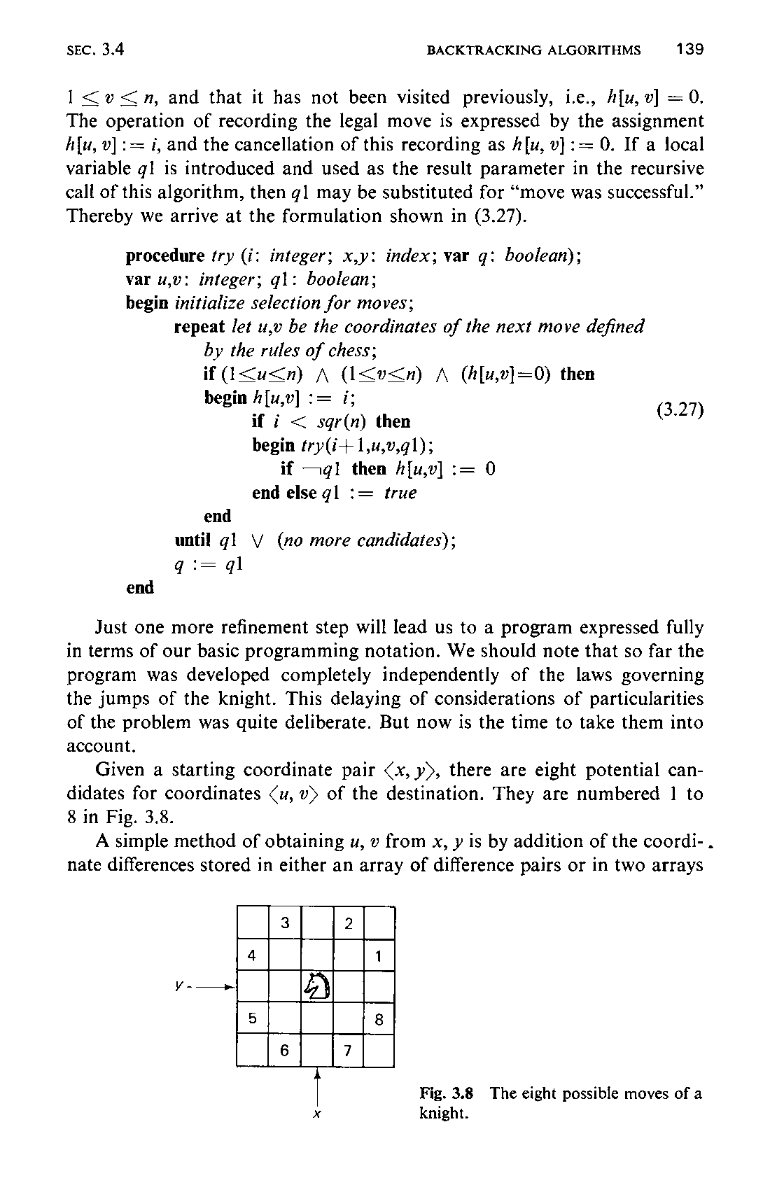
Which statements can now be refined on the basis of these decisions? Certainly “board not full” can be expressed as “i < n?.” Moreover, if we introduce two local variables wu and v to stand for the coordinates of possible move destinations determined according to the jump pattern of knights, then the predicate “acceptable” can be expressed as the logical combination of the conditions that the new field lies on the board, i.e., 1 << u<n and139 1 <v <n, and that it has not been visited previously, i.e., A{u, v] = 0. The operation of recording the legal move is expressed by the assignment A[u, v] := i, and the cancellation of this recording as /[u, v] := 0. If a local variable q1 is introduced and used as the result parameter in the recursive call of this algorithm, then g1 may be substituted for “move was successful.” Thereby we arrive at the formulation shown in (3.27).

Just one more refinement step will lead us to a program expressed fully in terms of our basic programming notation. We should note that so far the program was developed completely independently of the laws governing the jumps of the knight. This delaying of considerations of particularities of the problem was quite deliberate. But now is the time to take them into account.

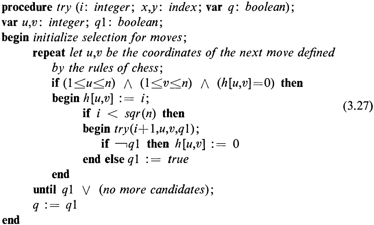
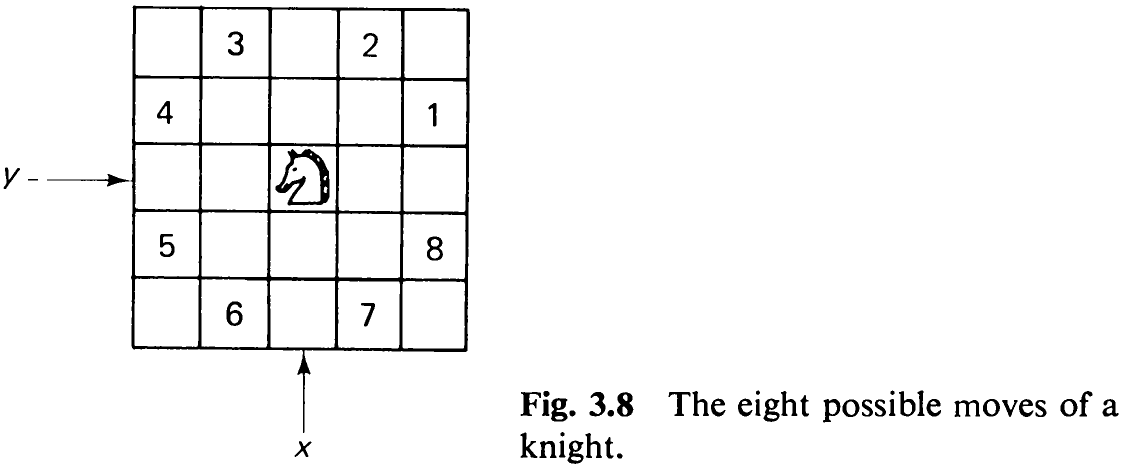
Given a starting coordinate pair <x, y>, there are eight potential candidates for coordinates <u, v> of the destination. They are numbered | to 8 in Fig. 3.8.

A simple method of obtaining u, v from x, y is by addition of the coordi- . nate differences stored in either an array of difference pairs or in two arrays

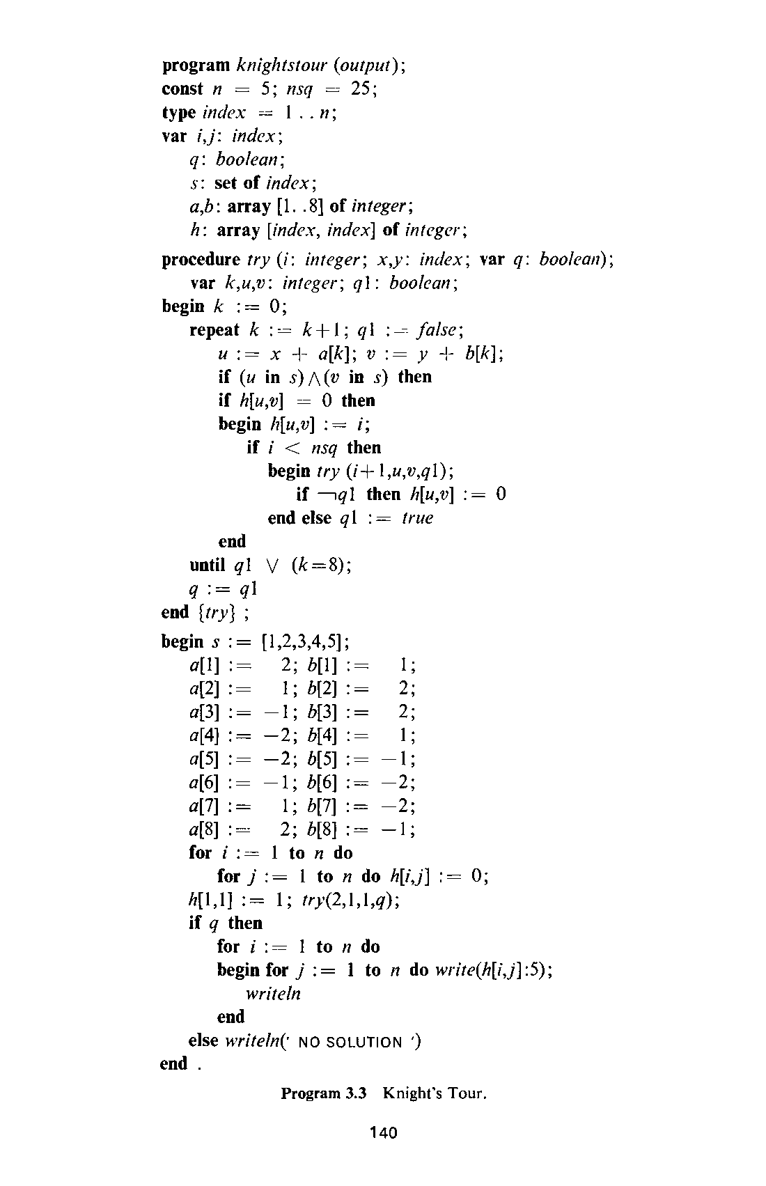
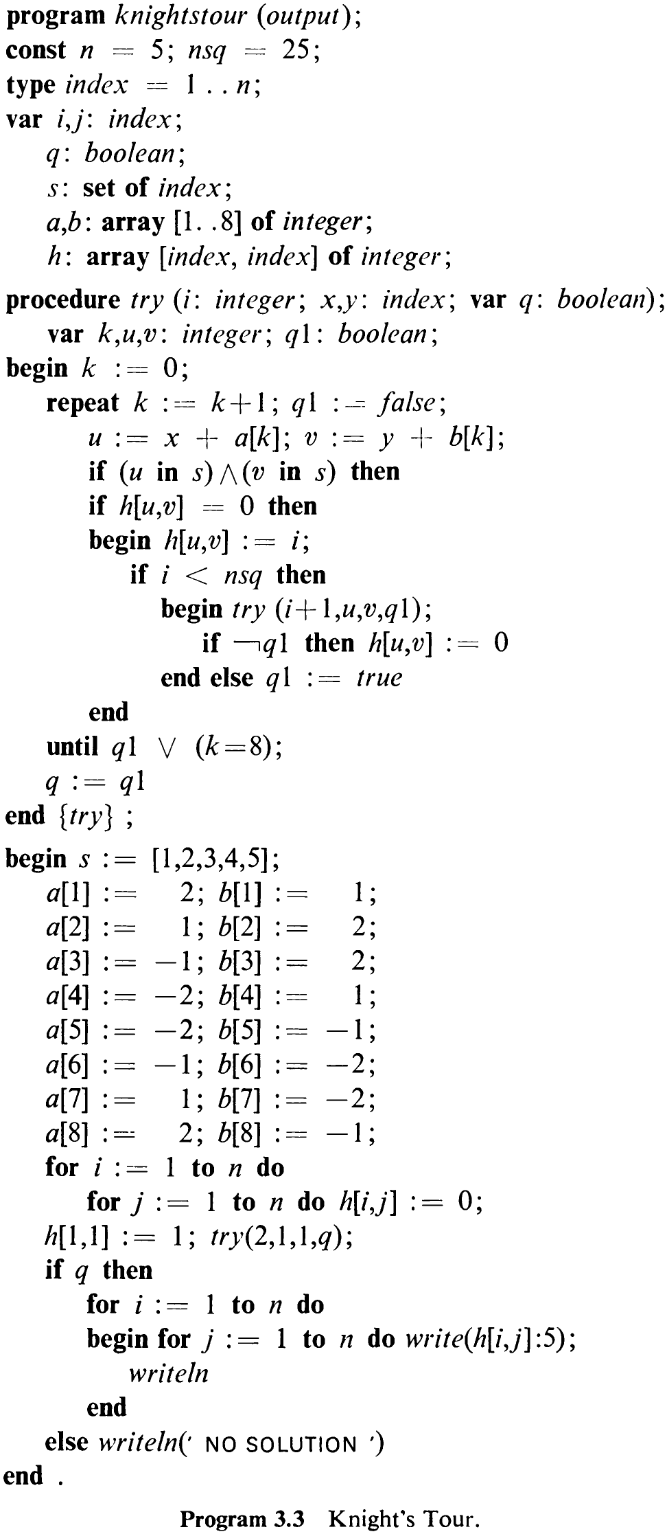
of single differences. Let these arrays be denoted by a and 5, appropriately initialized. Then an index k may be used to number the “next candidate.” The details are shown in Program 3.3. The recursive procedure is initiated by a call with the coordinates x9, yy of that field as parameters, from which the tour is to start. This field must be given the value 1; all others are to be marked free.

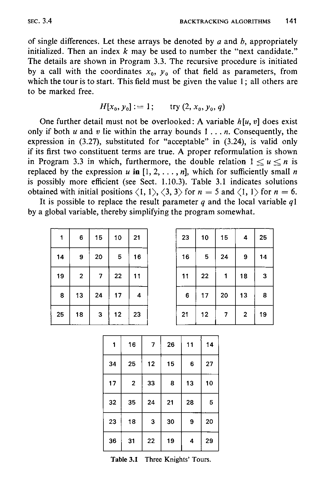
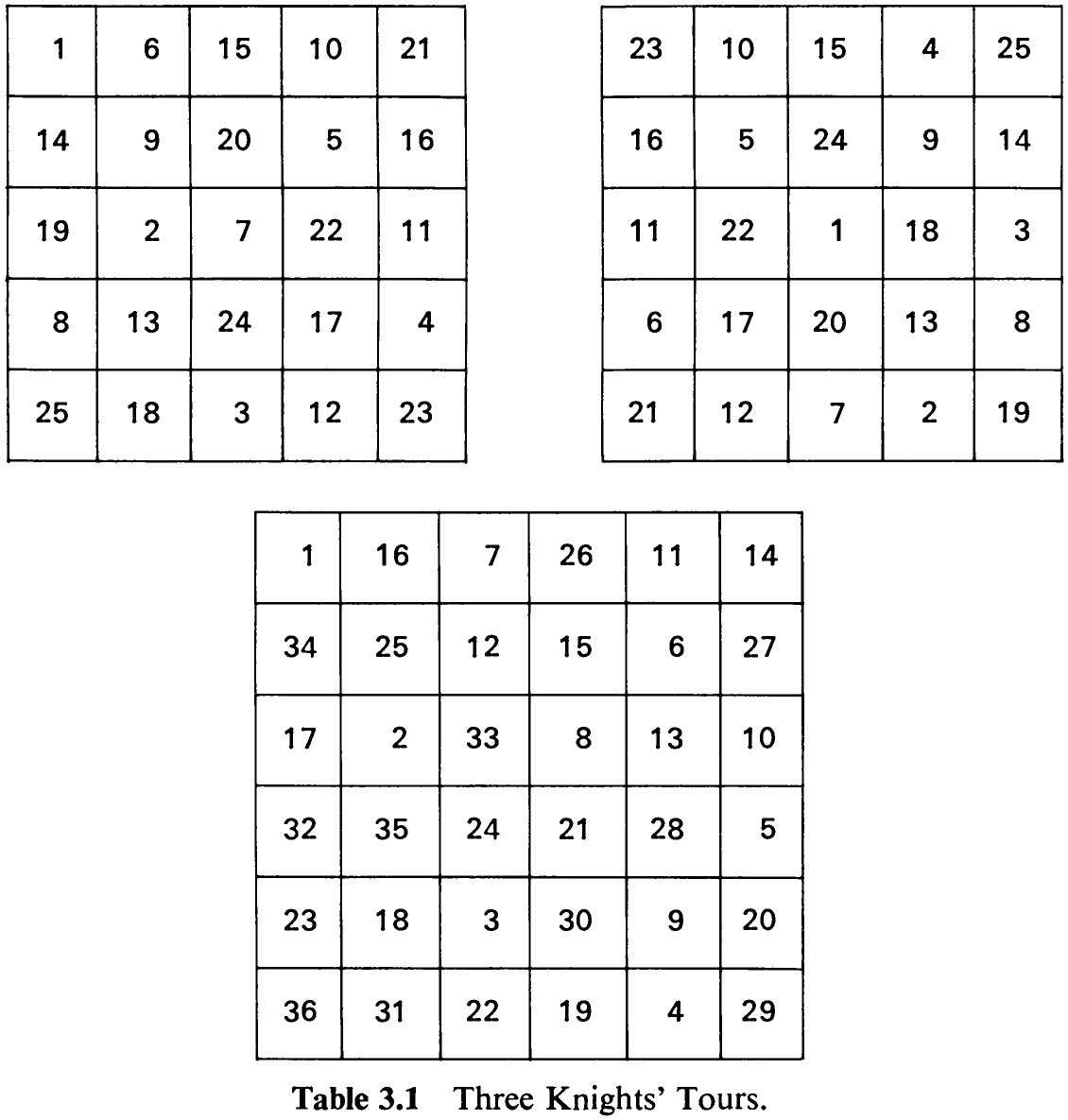
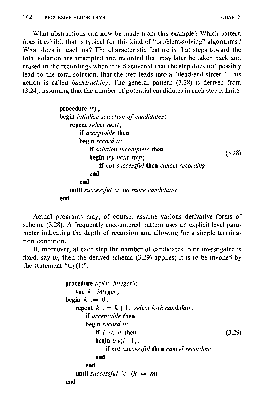
One further detail must not be overlooked: A variable h[u, v] does exist only if both uw and v lie within the array bounds 1... n. Consequently, the expression in (3.27), substituted for “acceptable” in (3.24), is valid only if its first two constituent terms are true. A proper reformulation is shown in Program 3.3 in which, furthermore, the double relation 1 <u<n is replaced by the expression wu in [1, 2,...,m], which for sufficiently small n is possibly more efficient (see Sect. 1.10.3). Table 3.1 indicates solutions obtained with initial positions <1, 15, <3, 3> for n = 5 and <1, 1> forn = 6.

It is possible to replace the result parameter q and the local variable q1 by a global variable, thereby simplifying the program somewhat.

What abstractions can now be made from this example? Which pattern does it exhibit that is typical for this kind of “problem-solving” algorithms ? What does it teach us? The characteristic feature is that steps toward the total solution are attempted and recorded that may later be taken back and erased in the recordings when it is discovered that the step does not possibly lead to the total solution, that the step leads into a “dead-end street.” This action is called backtracking. The general pattern (3.28) is derived from (3.24), assuming that the number of potential candidates in each step is finite.

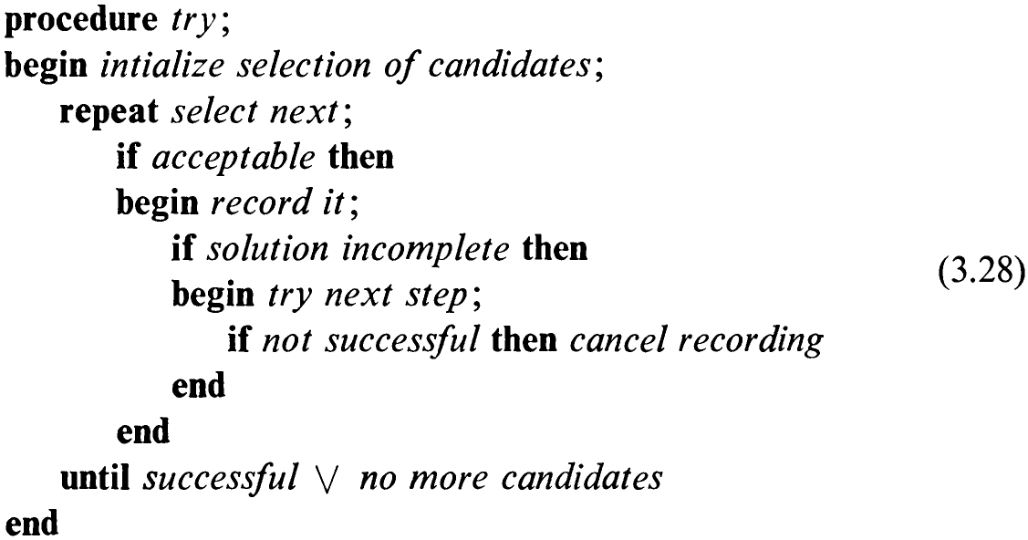
Actual programs may, of course, assume various derivative forms of schema (3.28). A frequently encountered pattern uses an explicit level parameter indicating the depth of recursion and allowing for a simple termination condition.

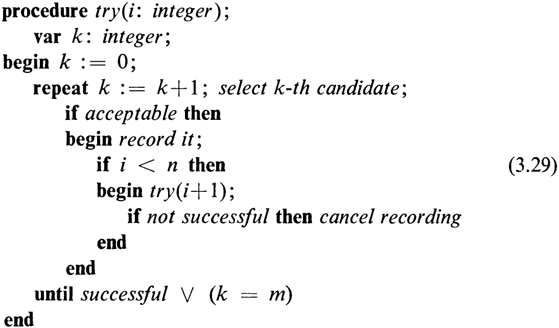
If, moreover, at each step the number of candidates to be investigated is fixed, say m, then the derived schema (3.29) applies; it is to be invoked by the statement “try(1)”.

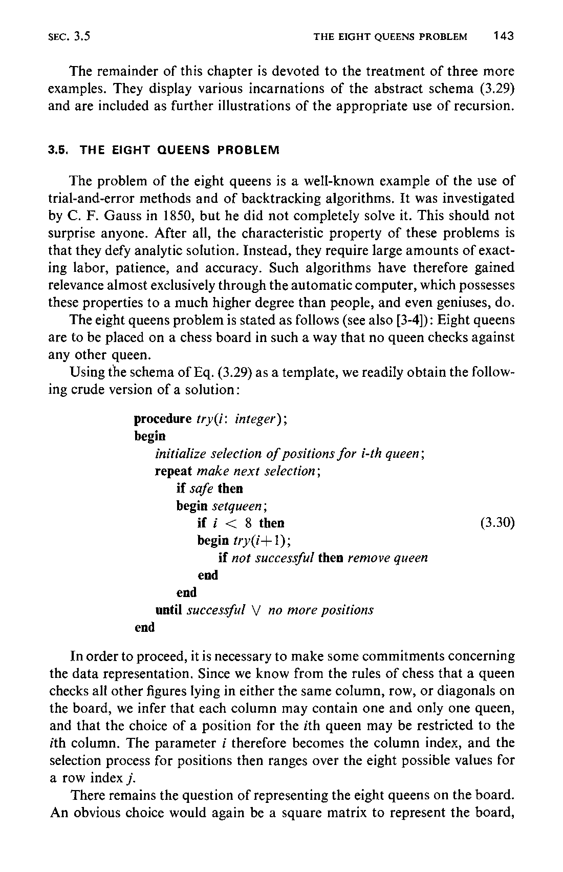
The remainder of this chapter is devoted to the treatment of three more examples. They display various incarnations of the abstract schema (3.29) and are included as further illustrations of the appropriate use of recursion.