Linear Lists

4.3.1 Basic Operations

The simplest way to interrelate or link a set of elements is to line them up in a single list or queue. For, in this case, only a single link is needed for each element to refer to its successor.

Assume that a type T is defined as shown in (4.11). Every variable of this type consists of three components, namely, an identifying key, the pointer to its successor, and possibly further associated information omitted in (4.11).

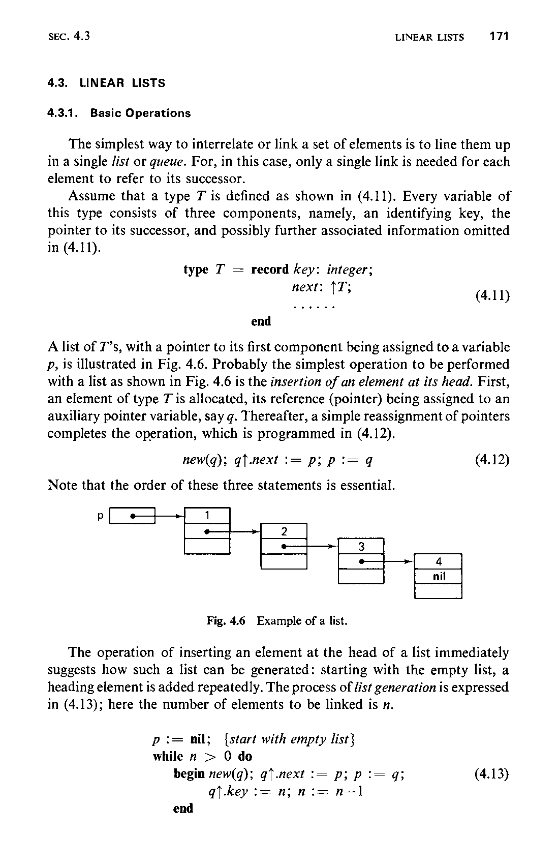
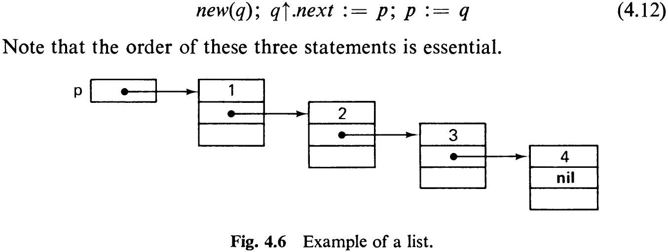
A list of T’s, with a pointer to its first component being assigned to a variable P, is illustrated in Fig. 4.6. Probably the simplest operation to be performed with a list as shown in Fig. 4.6 is the insertion of an element at its head. First, an element of type T is allocated, its reference (pointer) being assigned to an auxiliary pointer variable, say g. Thereafter, a simple reassignment of pointers completes the operation, which is programmed in (4.12).

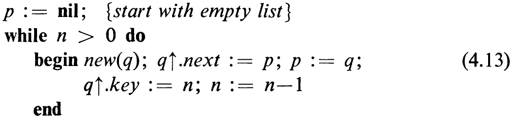
The operation of inserting an element at the head of a list immediately suggests how such a list can be generated: starting with the empty list, a heading element is added repeatedly. The process of list generation is expressed in (4.13); here the number of elements to be linked is n.

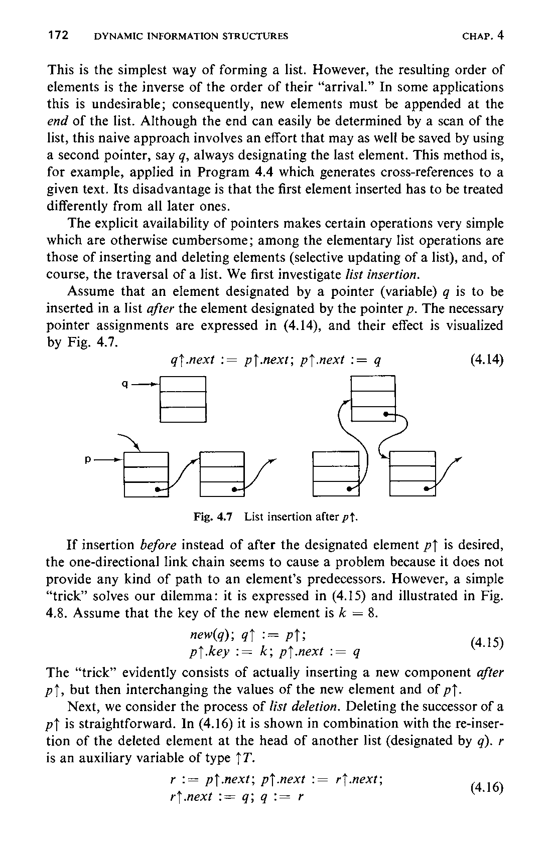
This is the simplest way of forming a list. However, the resulting order of elements is the inverse of the order of their “arrival.” In some applications this is undesirable; consequently, new elements must be appended at the end of the list. Although the end can easily be determined by a scan of the list, this naive approach involves an effort that may as well be saved by using a second pointer, say q, always designating the last element. This method is, for example, applied in Program 4.4 which generates cross-references to a given text. Its disadvantage is that the first element inserted has to be treated differently from all later ones.

The explicit availability of pointers makes certain operations very simple which are otherwise cumbersome; among the elementary list operations are those of inserting and deleting elements (selective updating of a list), and, of course, the traversal of a list. We first investigate list insertion.

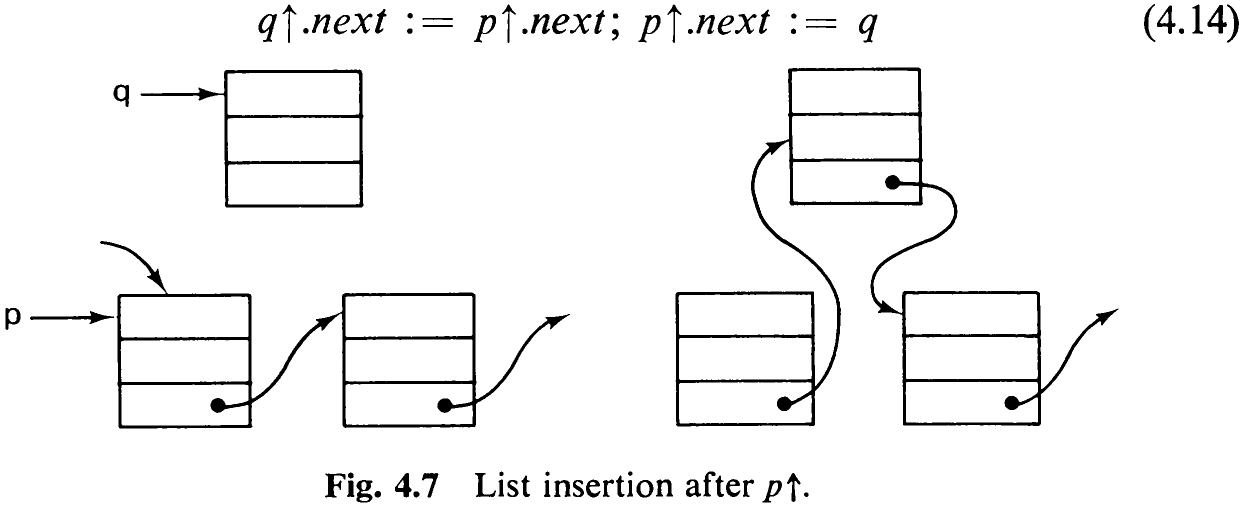
Assume that an element designated by a pointer (variable) g is to be inserted in a list after the element designated by the pointer p. The necessary pointer assignments are expressed in (4.14), and their effect is visualized by Fig. 4.7.

If insertion before instead of after the designated element pf is desired, the one-directional link chain seems to cause a problem because it does not provide any kind of path to an element’s predecessors. However, a simple “trick” solves our dilemma: it is expressed in (4.15) and illustrated in Fig. 4.8. Assume that the key of the new element is k = 8.

The “trick” evidently consists of actually inserting a new component after p}, but then interchanging the values of the new element and of p7.

Next, we consider the process of /Jist deletion. Deleting the successor of a pt is straightforward. In (4.16) it is shown in combination with the re-insertion of the deleted element at the head of another list (designated by q). r is an auxiliary variable of type TT.

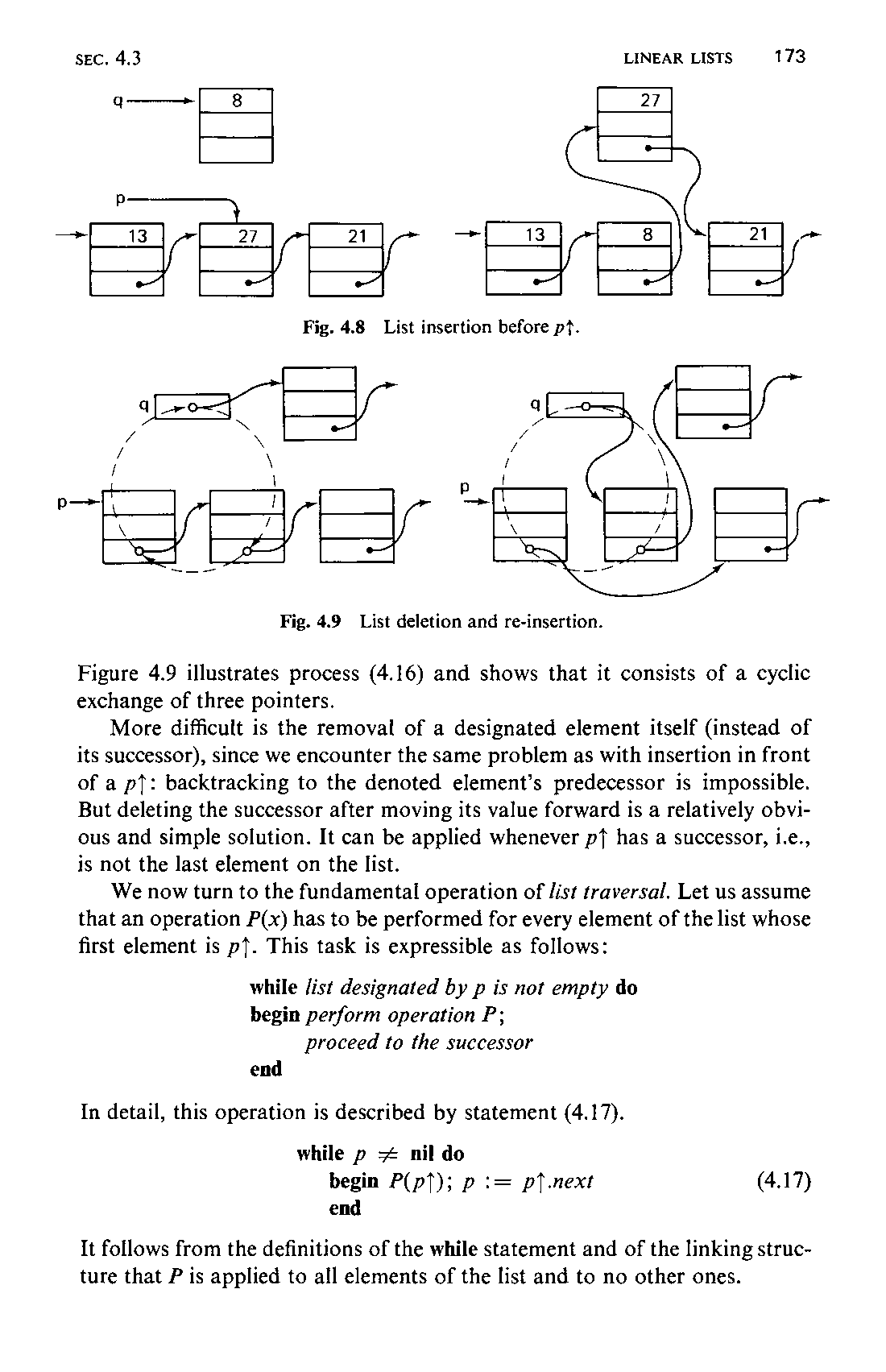
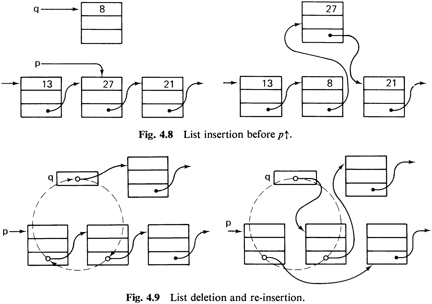
Figure 4.9 illustrates process (4.16) and shows that it consists of a cyclic exchange of three pointers.

More difficult is the removal of a designated element itself (instead of its successor), since we encounter the same problem as with insertion in front of a pt: backtracking to the denoted element’s predecessor is impossible. But deleting the successor after moving its value forward is a relatively obvious and simple solution. It can be applied whenever p} has a successor, i.e., is not the last element on the list.

We now turn to the fundamental operation of Jist traversal. Let us assume that an operation P(x) has to be performed for every element of the list whose first element is pt. This task is expressible as follows:

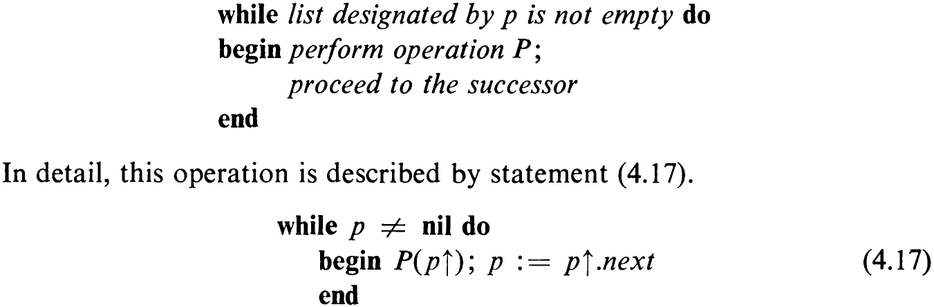
It follows from the definitions of the while statement and of the linking structure that P is applied to all elements of the list and to no other ones.

A very frequent operation performed is list searching for an element with a given key x. As with file structures, the search is purely sequential. The search terminates either if an element is found or if the end of the list is reached. Again, we assume that the head of the list is designated by a pointer p. A first attempt to formulate this simple search results in the following:

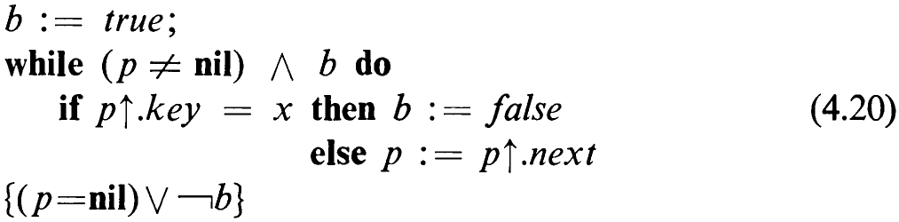
However, it must be noticed that P = nil implies that pt does not exist. Hence, evaluation of the termination condition may imply access to a nonexisting variable (in contrast to a variable with undefined value) and may cause failure of program execution. This can be remedied either by using an explicit break of the repetition expressed by a goto statement (4.19) or by introducing an auxiliary Boolean variable to record whether or not a desired key was found (4.20).

The use of the goto statement requires the presence of a destination label at some place; note that its incompatibility with the while statement is evidenced by the fact that the while clause becomes misleading: the controlled statement is not necessarily executed as long as p + nil.

4.3.2 Ordered Lists and Re-organizing Lists

Algorithm (4.20) strongly recalls the search routines for scanning an array or a file. In fact, a file is nothing but a linear list in which the technique of linkage to the successor is left unspecified or implicit. Since the primitive file operators do not allow insertion of new elements (except at the end) or deletion (except removal of all elements), the choice of representation is left wide open to the implementor, and he may well use sequential allocation, leaving successive components in contiguous storage areas. Linear lists with explicit pointers provide more flexibility, and therefore they should be used whenever this additional flexibility is needed.

To exemplify, we will now consider a problem that will re-occur throughout this chapter in order to illustrate alternative solutions and techniques. It is the problem of reading a text, collecting all its words, and counting the frequency of their occurrence. It is called the construction of a concordance.

175 An obvious solution is to construct a list of words found in the text. The list is scanned for each word. If the word is found, its frequency count is incremented; otherwise the word is added to the list. We shall simply call this process search, although it may apparently also include an insertion.

In order to be able to concentrate our attention on the essential part of list handling, we assume that the words have already been extracted from the text under investigation, have been encoded as integers, and are available in the form of an input file.

The formulation of the procedure called search follows in a straightforward manner from (4.20). The variable root refers to the head of the list in which new words are inserted according to (4.12). The complete algorithm is listed as Program 4.1; it includes a routine for tabulating the constructed concordance list. The tabulation process is an example in which an action is executed once for each element of the list, as shown in schematic form in (4.17).

program list (input,output);
{straight list insertion}
  type ref = ↑word;
    word = record key: integer;
                  count: integer;
                  next: ref
           end ;
  var k: integer; root: ref;

  procedure search (x: integer; var root: ref);
    var w: ref; b: boolean;
  begin w := root; b := true;
    while (w≠nil) ∧ b do
      if w↑.key = x then b := false else w := w↑.next;
    if b then
    begin {new entry} w := root; new (root);
      with root↑ do
      begin key := x; count := 1; next := w
      end
    end else
    w↑.count := w↑.count + 1
  end {search} ;

  procedure printlist (w: ref);
  begin while w ≠ nil do
        begin writeln (w↑.key, w↑.count);
              w := w↑.next
        end
  end {printlist} ;
begin root := nil; read(k);
  while k ≠ 0 do
    begin search (k, root); read(k)
    end ;
  printlist(root)
end .

The linear scan algorithm of Program 4.1 recalls the search procedure for arrays and files, and in particular the simple technique used to simplify the loop termination condition: the use of a sentinel. A sentinel may as well176 be used in list search; it is represented by a dummy element at the end of the list. The new procedure is (4.21), which replaces the search procedure of Program 4.1, provided that a global variable sentinel is added and that the initialization of root is replaced by the statements

new(sentinel); root := sentinel;

which generate the element to be used as sentinel.

procedure search(x: integer; var root: ref);
  var w: ref;
begin w := root; sentinel↑.key := x;
  while w↑.key ≠ x do w := w↑.next;
  if w ≠ sentinel then w↑.count := w↑.count + 1 else
    begin {new entry} w := root; new(root);
      with root↑ do
      begin key := x; count := 1; next := w
      end
    end
end {search}

Obviously, the power and flexibility of the linked list are ill used in this example, and the linear scan of the entire list can only be accepted in cases in which the number of elements is limited. An easy improvement, however, is readily at hand: the ordered list search. If the list is ordered (say by increasing keys), then the search may be terminated at the latest upon encountering the first key which is larger than the new one. Ordering of the list is achieved by inserting new elements at the appropriate place instead of at the head. In effect, ordering is practically obtained free of charge. This is because of the ease by which insertion in a linked list is achieved, i.e., by making full use of its flexibility. It is a possibility not provided by the array and file structures.177 (Note, however, that even in ordered lists no equivalent to the binary search of arrays is available.)

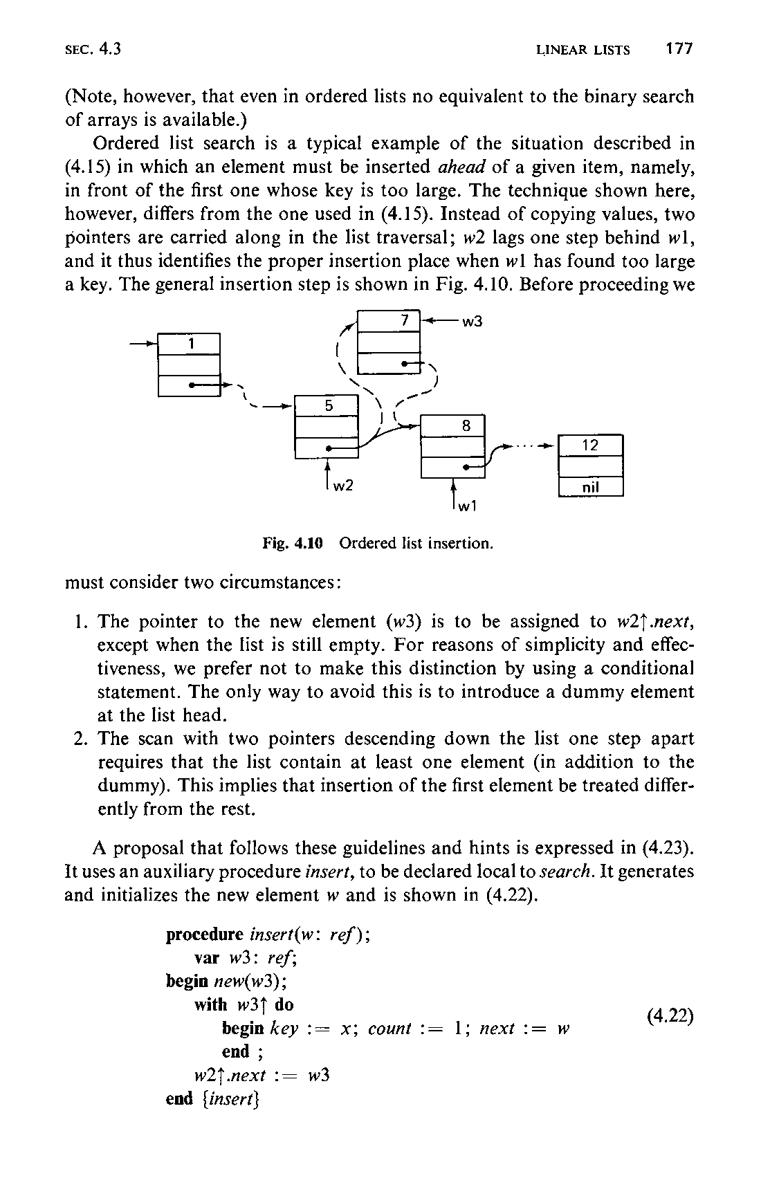
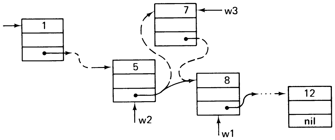
Ordered list search is a typical example of the situation described in (4.15) in which an element must be inserted ahead of a given item, namely, in front of the first one whose key is too large. The technique shown here, however, differs from the one used in (4.15). Instead of copying values, two pointers are carried along in the list traversal; w2 lags one step behind w1, and it thus identifies the proper insertion place when w1 has found too large a key. The general insertion step is shown in Fig. 4.10. Before proceeding we must consider two circumstances:

1. The pointer to the new element (w3) is to be assigned to w2↑.next, except when the list is still empty. For reasons of simplicity and effectiveness, we prefer not to make this distinction by using a conditional statement. The only way to avoid this is to introduce a dummy element at the list head.
2. The scan with two pointers descending down the list one step apart requires that the list contain at least one element (in addition to the dummy). This implies that insertion of the first element be treated differently from the rest.

A proposal that follows these guidelines and hints is expressed in (4.23). It uses an auxiliary procedure insert, to be declared local to search. It generates and initializes the new element $w$ and is shown in (4.22).

procedure insert(w: ref);
  var w3: ref;
begin new(w3);
  with w3↑ do
    begin key := x; count := 1; next := w
    end ;
  w2↑.next := w3
end {insert}

178 The initializing statement “root := nil” in Program 4.1 is accordingly replaced by

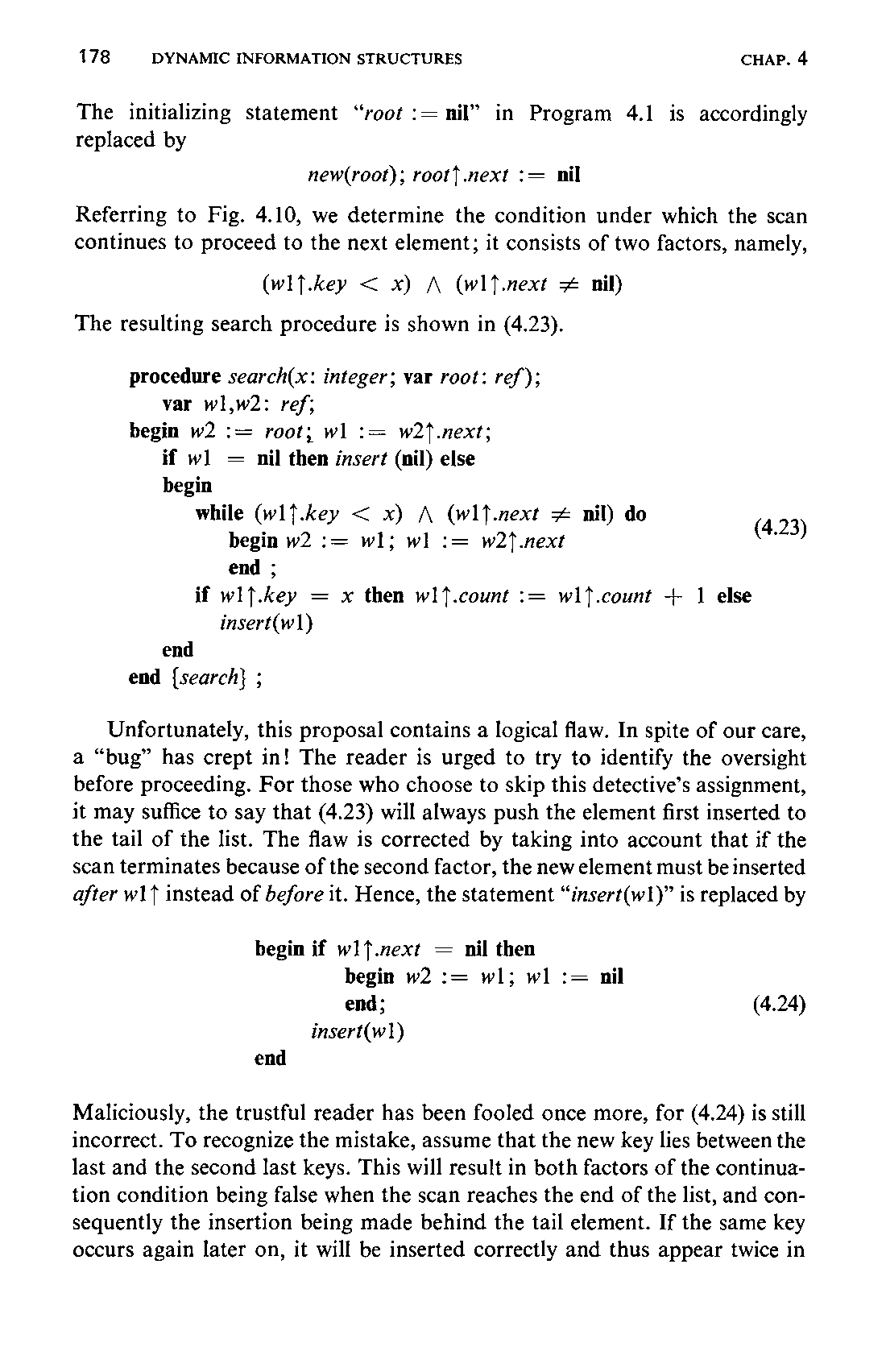
new(root); root↑.next := nil

Referring to Fig. 4.10, we determine the condition under which the scan continues to proceed to the next element; it consists of two factors, namely,

(w1↑.key < x) ∧ (w1↑.next ≠ nil)

The resulting search procedure is shown in (4.23).

procedure search(x: integer; var root: ref);
  var w1,w2: ref;
begin w2 := root; w1 := w2↑.next;
  if w1 = nil then insert (nil) else
  begin
    while (w1↑.key < x) ∧ (w1↑.next ≠ nil) do
      begin w2 := w1; w1 := w2↑.next
      end ;
    if w1↑.key = x then w1↑.count := w1↑.count + 1 else
       insert(w1)
  end
end {search} ;

Unfortunately, this proposal contains a logical flaw. In spite of our care, a “bug” has crept in! The reader is urged to try to identify the oversight before proceeding. For those who choose to skip this detective’s assignment, it may suffice to say that (4.23) will always push the element first inserted to the tail of the list. The flaw is corrected by taking into account that if the scan terminates because of the second factor, the new element must be inserted after w1↑ instead of before it. Hence, the statement “insert(w1)” is replaced by

begin if w1↑.next = nil then
         begin w2 := w1; w1 := nil
         end;
      insert(w1)
end

Maliciously, the trustful reader has been fooled once more, for (4.24) is still incorrect. To recognize the mistake, assume that the new key lies between the last and the second last keys. This will result in both factors of the continuation condition being false when the scan reaches the end of the list, and consequently the insertion being made behind the tail element. If the same key occurs again later on, it will be inserted correctly and thus appear twice in179 the tabulation. The remedy lies in replacing the condition

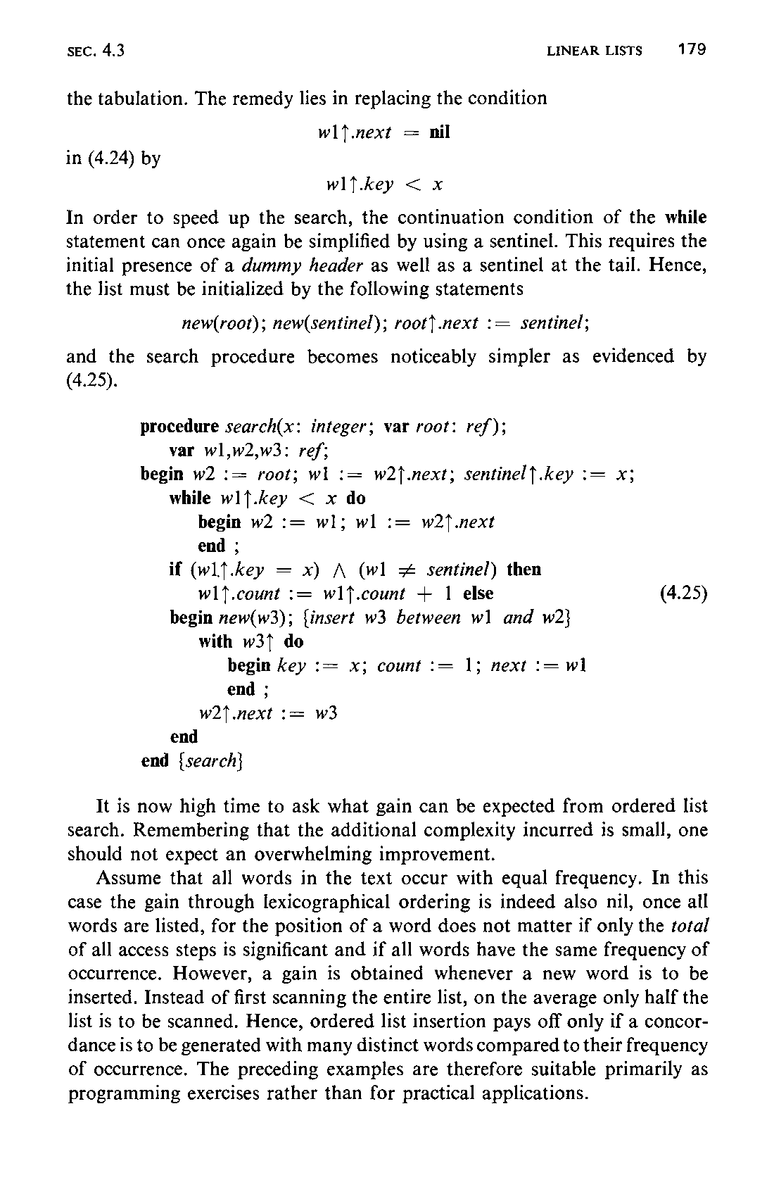
w1↑.next = nil

in (4.24) by

w1↑.key < x

In order to speed up the search, the continuation condition of the while statement can once again be simplified by using a sentinel. This requires the initial presence of a dummy header as well as a sentinel at the tail. Hence, the list must be initialized by the following statements

new(root); new(sentinel); root↑.next := sentinel;

and the search procedure becomes noticeably simpler as evidenced by (4.25).

procedure search(x: integer; var root: ref);
  var w1,w2,w3: ref;
begin w2 := root; w1 := w2↑.next; sentinel↑.key := x;
  while w1↑.key < x do
    begin w2 := w1; w1 := w2↑.next
    end ;
  if (w1↑.key = x) ∧ (w1 ≠ sentinel) then
    w1↑.count := w1↑.count + 1 else
  begin new(w3); {insert w3 between w1 and w2}
    with w3↑ do
      begin key := x; count := 1; next := w1
      end ;
    w2↑.next := w3
  end
end {search}

It is now high time to ask what gain can be expected from ordered list search. Remembering that the additional complexity incurred is small, one should not expect an overwhelming improvement.

Assume that all words in the text occur with equal frequency. In this case the gain through lexicographical ordering is indeed also nil, once all words are listed, for the position of a word does not matter if only the total of all access steps is significant and if all words have the same frequency of occurrence. However, a gain is obtained whenever a new word is to be inserted. Instead of first scanning the entire list, on the average only half the list is to be scanned. Hence, ordered list insertion pays off only if a concordance is to be generated with many distinct words compared to their frequency of occurrence. The preceding examples are therefore suitable primarily as programming exercises rather than for practical applications.

180 The arrangement of data in a linked list is recommended when the number of elements is relatively small (say $< 100$), varies, and, moreover, when no information is given about their frequencies of access. A typical example is the symbol table in compilers of programming languages. Each declaration causes the addition of a new symbol, and upon exit from its scope of validity, it is deleted from the list. The use of simple linked lists is appropriate for applications with relatively short programs. Even in this case a considerable improvement in access method can be achieved by a very simple technique which is mentioned here again primarily because it constitutes a pretty example for demonstrating the flexibilities of the linked list structure.

A characteristic property of programs is that occurrences of the same identifier are very often clustered, that is, one occurrence is often followed by one or more re-occurrences of the same word. This information is an invitation to re-organize the list after each access by moving the word that was found to the top of the list, thereby minimizing the length of the search path the next time it is sought. This method of access is called list search with re-ordering, or—somewhat pompously—self-organizing list search. In presenting the corresponding algorithm in the form of a procedure which may be substituted in Program 4.1, we take advantage of our experience made so far and introduce a sentinel right from the start. In fact, a sentinel not only speeds up the search, but in this case it also simplifies the program. The list is, however, not initially empty, but contains the sentinel element already. The initial statements are

new (sentinel); root := sentinel;

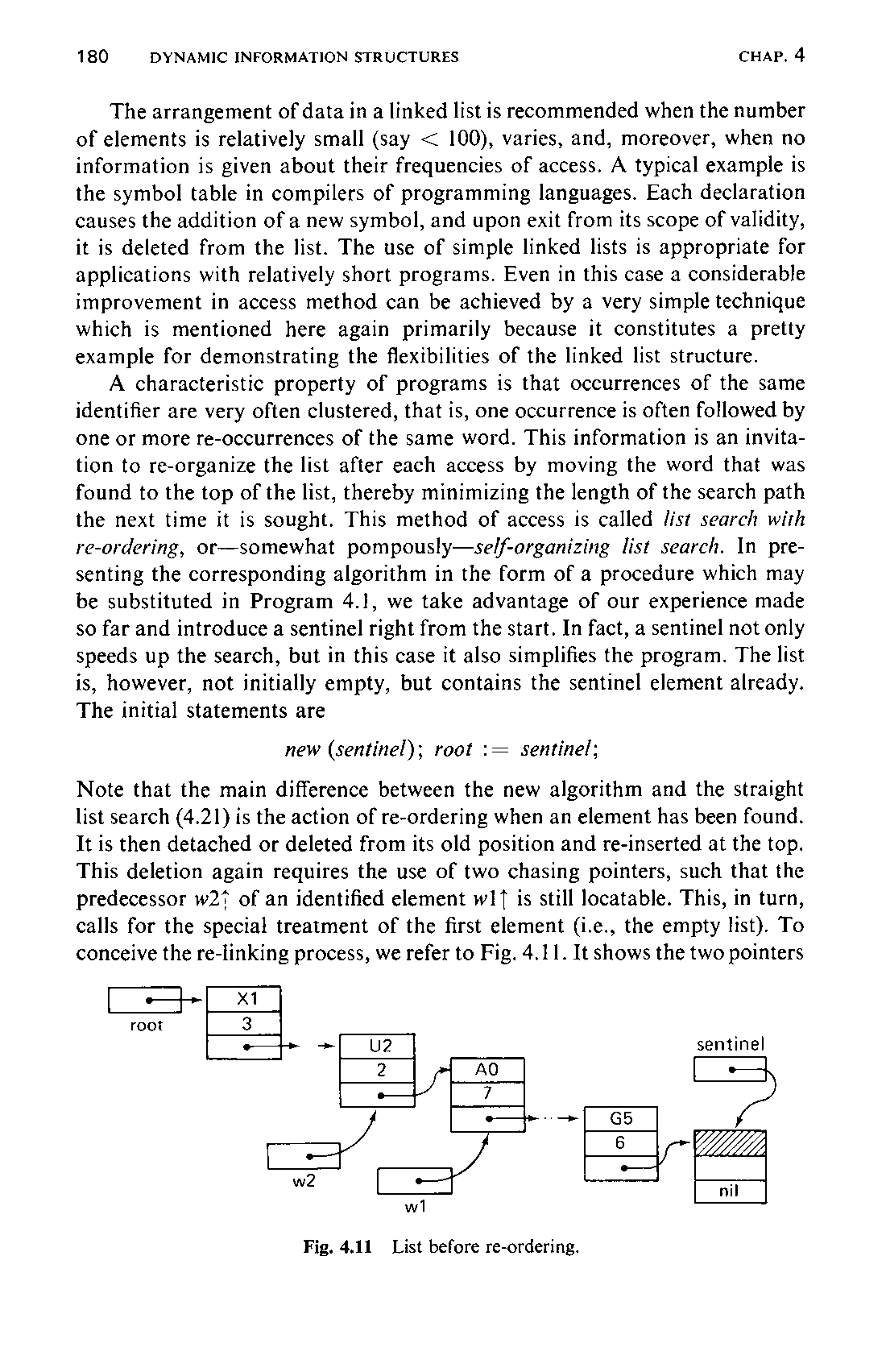
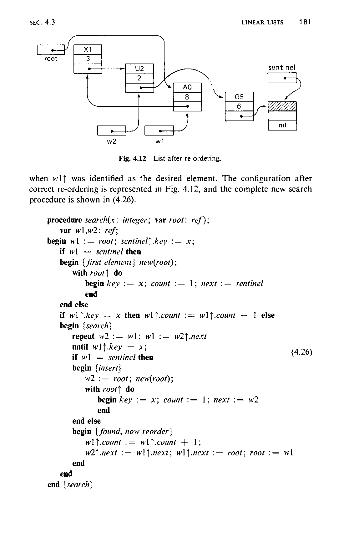
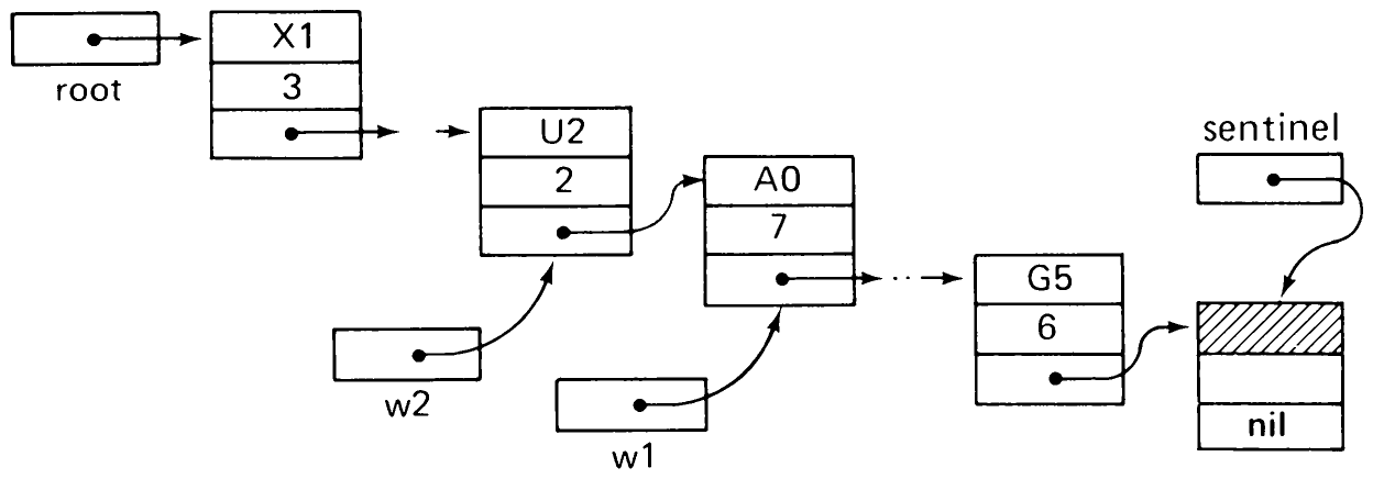
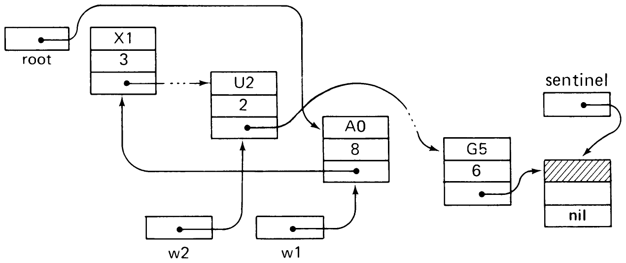
Note that the main difference between the new algorithm and the straight list search (4.21) is the action of re-ordering when an element has been found. It is then detached or deleted from its old position and re-inserted at the top. This deletion again requires the use of two chasing pointers, such that the predecessor w2↑ of an identified element w1↑ is still locatable. This, in turn, calls for the special treatment of the first element (i.e., the empty list). To conceive the re-linking process, we refer to Fig. 4.11. It shows the two pointers181 when w1↑ was identified as the desired element. The configuration after correct re-ordering is represented in Fig. 4.12, and the complete new search procedure is shown in (4.26).

procedure search(x: integer; var root: ref);
  var w1,w2: ref;
begin w1 := root; sentinel↑.key := x;
  if w1 = sentinel then
  begin {first element} new(root);
    with root↑ do
      begin key := x; count := 1; next := sentinel
      end
  end else
  if w1↑.key = x then w1↑.count := w1↑.count + 1 else
  begin {search}
    repeat w2 := w1; w1 := w2↑.next
    until w1↑.key = x;
    if w1 = sentinel then
    begin {insert}
      w2 := root; new(root);
      with root↑ do
        begin key := x; count := 1; next := w2
        end
    end else
    begin {found, now reorder}
      w1↑.count := w1↑.count + 1;
      w2↑.next := w1↑.next; w1↑.next := root; root := w1
    end
  end
end {search}

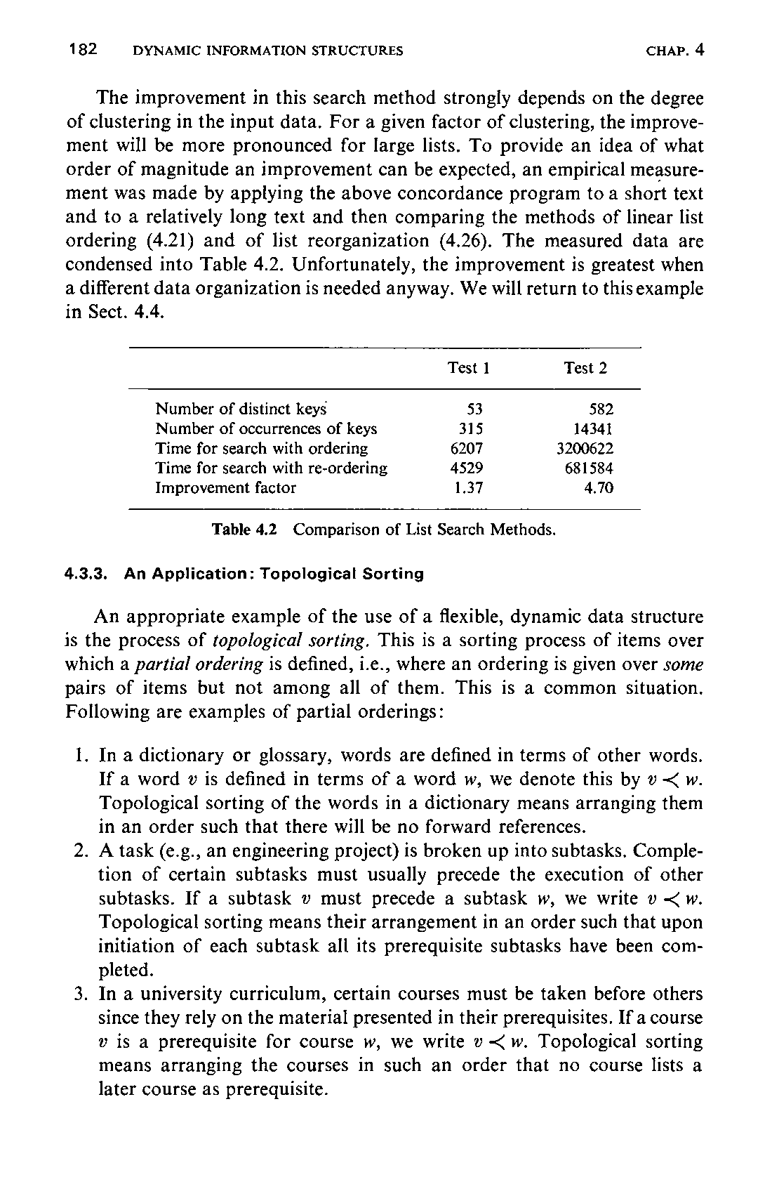
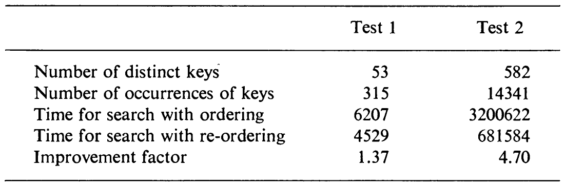
182 The improvement in this search method strongly depends on the degree of clustering in the input data. For a given factor of clustering, the improvement will be more pronounced for large lists. To provide an idea of what order of magnitude an improvement can be expected, an empirical measurement was made by applying the above concordance program to a short text and to a relatively long text and then comparing the methods of linear list ordering (4.21) and of list reorganization (4.26). The measured data are condensed into Table 4.2. Unfortunately, the improvement is greatest when a different data organization is needed anyway. We will return to this example in Sect. 4.4.

4.3.3 An Application: Topological Sorting

An appropriate example of the use of a flexible, dynamic data structure is the process of topological sorting. This is a sorting process of items over which a partial ordering is defined, i.e., where an ordering is given over some pairs of items but not among all of them. This is a common situation. Following are examples of partial orderings:

1. In a dictionary or glossary, words are defined in terms of other words. If a word $v$ is defined in terms of a word $w$, we denote this by $v \prec w$. Topological sorting of the words in a dictionary means arranging them in an order such that there will be no forward references.
2. A task (e.g., an engineering project) is broken up into subtasks. Completion of certain subtasks must usually precede the execution of other subtasks. If a subtask $v$ must precede a subtask $w$, we write $v \prec w$. Topological sorting means their arrangement in an order such that upon initiation of each subtask all its prerequisite subtasks have been completed.
3. In a university curriculum, certain courses must be taken before others since they rely on the material presented in their prerequisites. If a course $v$ is a prerequisite for course $w$, we write $v \prec w$. Topological sorting means arranging the courses in such an order that no course lists a later course as prerequisite.

183 4. In a program, some procedures may contain calls of other procedures. If a procedure $v$ is called by a procedure $w$, we write $v \prec w$. Topological sorting implies the arrangement of procedure declarations in such a way that there are no forward references.

In general, a partial ordering of a set $S$ is a relation between the elements of $S$. It is denoted by the symbol $\prec$, verbalized by “precedes,” and satisfies the following three properties (axioms) for any distinct elements $x$, $y$, and $z$ of $S$:

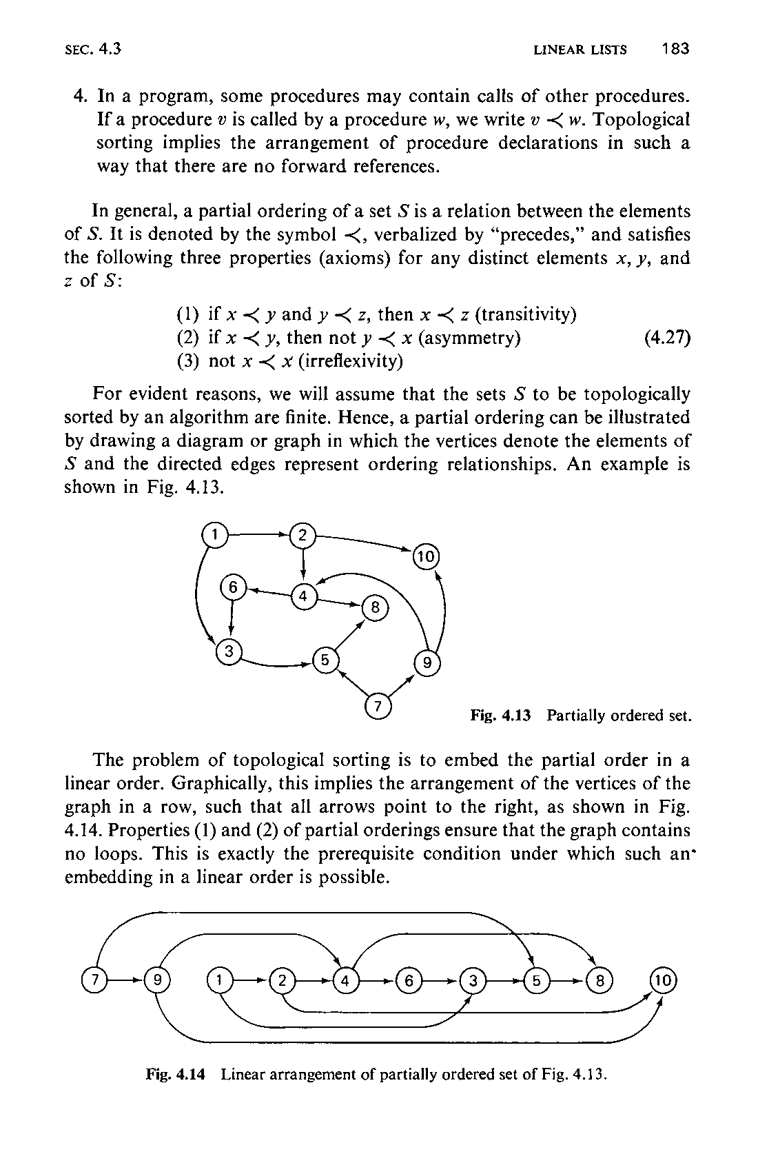
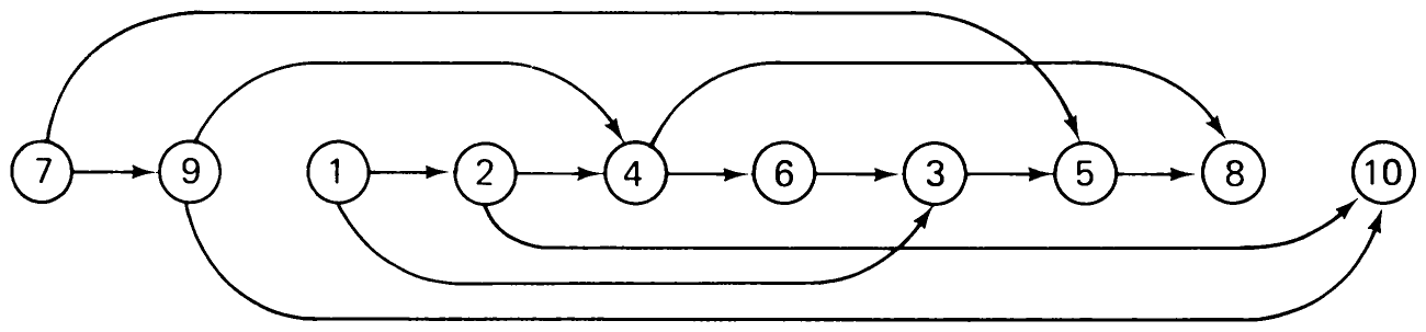
For evident reasons, we will assume that the sets $S$ to be topologically sorted by an algorithm are finite. Hence, a partial ordering can be illustrated by drawing a diagram or graph in which the vertices denote the elements of $S$ and the directed edges represent ordering relationships. An example is shown in Fig. 4.13.

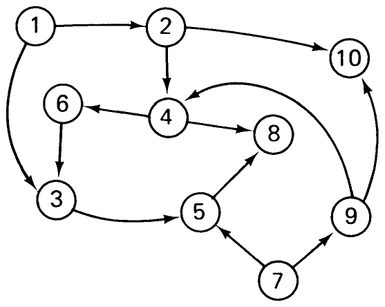
The problem of topological sorting is to embed the partial order in a linear order. Graphically, this implies the arrangement of the vertices of the graph in a row, such that all arrows point to the right, as shown in Fig. 4.14. Properties (1) and (2) of partial orderings ensure that the graph contains no loops. This is exactly the prerequisite condition under which such an embedding in a linear order is possible.

184 How do we proceed to find one of the possible linear orderings? The recipe is quite simple. We start by choosing any item that is not preceded by another item (there must be at least one; otherwise there would have to exist a loop). This object is placed at the head of the resulting list and removed from the set $S$. The remaining set is still partially ordered, and so the same algorithm can be applied again until the set is empty.

In order to describe this algorithm more rigorously, we must settle on a data structure and representation of $S$ and its ordering. The choice of this representation is determined by the operations to be performed, particularly the operation of selecting elements with zero predecessors. Every item should therefore be represented by three characteristics: its identification key, its set of successors, and a count of its predecessors. Since the number $n$ of elements in $S$ is not given a priori, the set is conveniently organized as a linked list. Consequently, an additional entry in the description of each item contains the link to the next item in the list. We will assume that the keys are integers (but not necessarily the consecutive integers from 1 to $n$). Analogously, the set of each item’s successors is conveniently represented as a linked list. Each element of the successor list is described by an identification and a link to the next item on this list. If we call the descriptors of the main list, in which each item of $S$ occurs exactly once, leaders, and the descriptors of elements on the successor chains trailers, we obtain the following declarations of data types:

type lref    = ↑leader;
     tref    = ↑trailer;
     leader  = record key, count: integer;
                 trail: tref;
                 next: lref
               end;
     trailer = record id: lref;
                 next: tref
               end

Assume that the set $S$ and its ordering relations are initially represented as a sequence of pairs of keys in the input file. The input data for the example in Fig. 4.13 are shown in (4.29) in which the symbols $\prec$ are added for the sake of clarity.

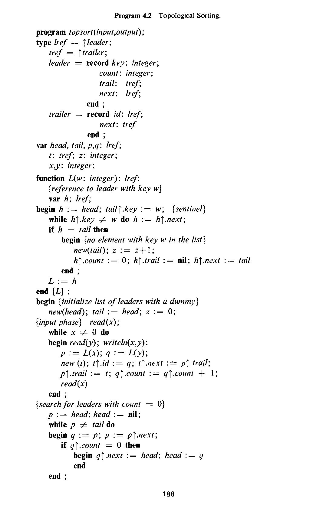
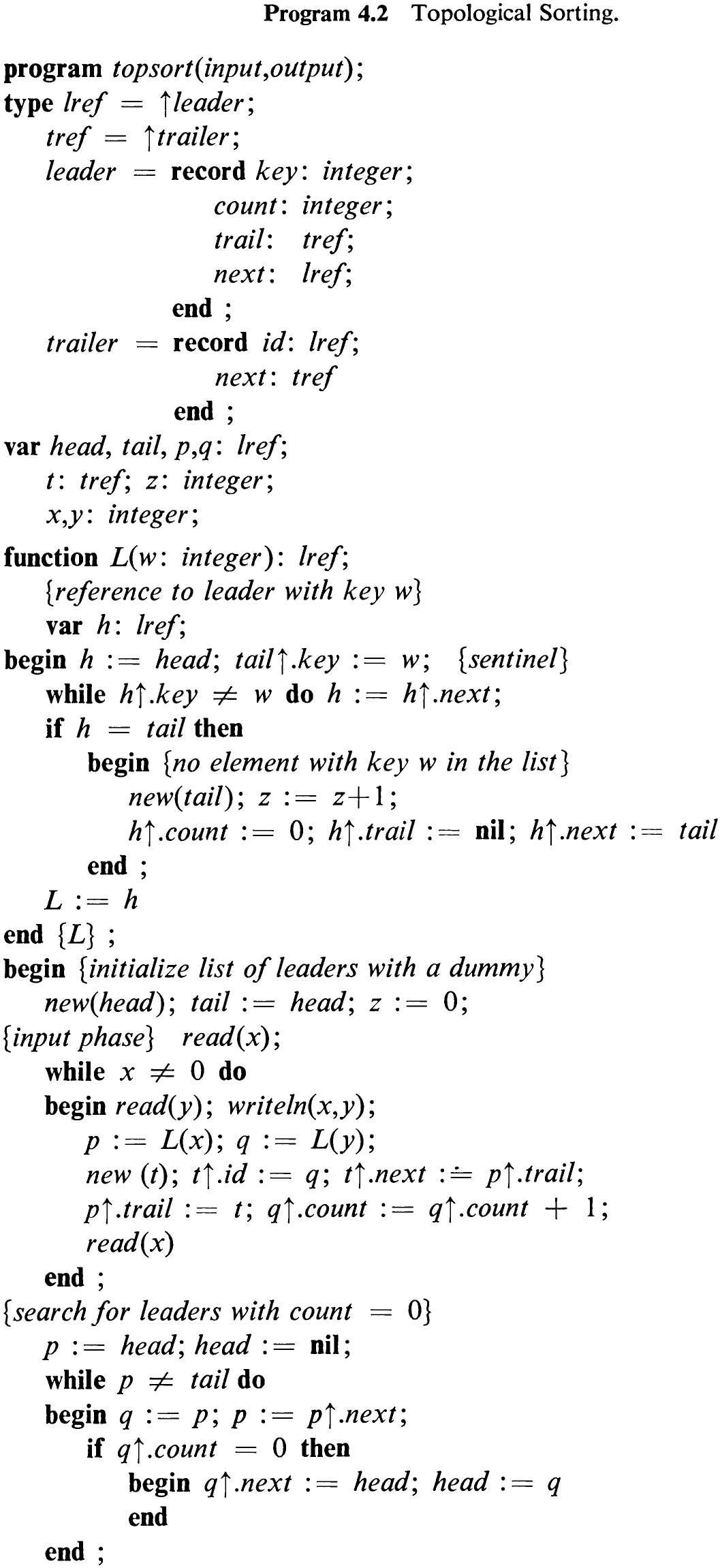
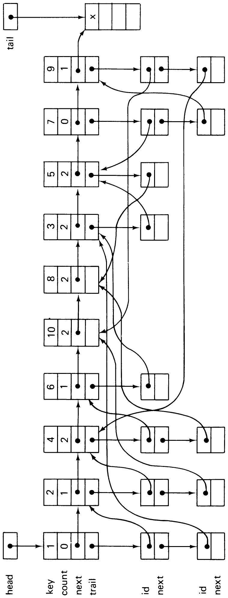
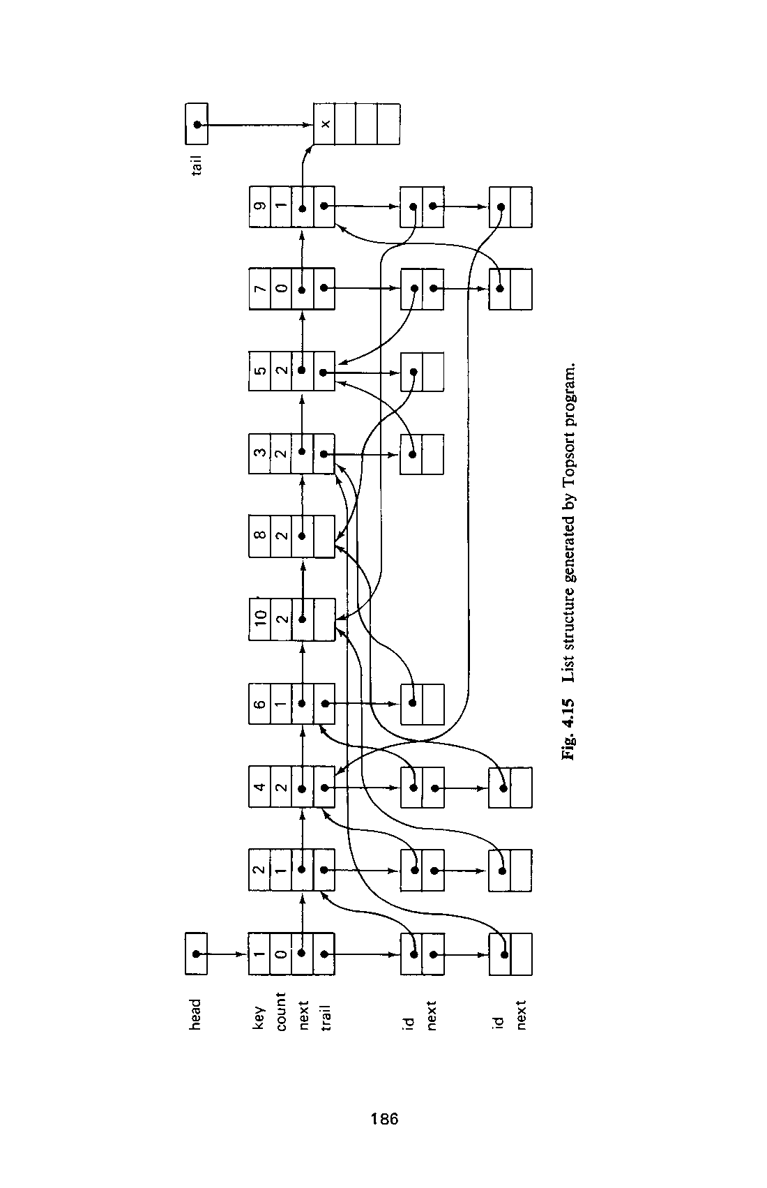
The first part of the topological sort program must read the input file and transform the data into a list structure. This is performed by successively reading a pair of keys $x$ and $y$ ($x \prec y$). Let us denote the pointers to their185 representations on the linked list of leaders by $p$ and $q$. These records must be located by a list search and, if not yet present, be inserted in the list. This task is performed by a function procedure called $L$. Subsequently, a new entry is added in the list of trailers of $x$, along with an identification of $y$; the count of predecessors of $y$ is incremented by 1. This algorithm is called input phase (4.30). Figure 4.15 illustrates the data structure generated during processing the input data (4.29) by (4.30) .This piece of program refers to a function $L(w)$ yielding the reference to the list component with key $w$ (see also Program 4.2). We assume that the sequence of input key pairs is terminated by an additional zero.

{input phase} read(x);
new(head); tail := head; z := 0;
while x ≠ 0 do
begin read(y); p := L(x); q := L(y);
  new(t); t↑.id := q; t↑.next := p↑.trail;
  p↑.trail := t; q↑.count := q↑.count + 1;
  read(x)
end

After the data structure of Fig. 4.15 has been constructed in this input phase, the actual process of topological sorting can be taken up as described above. But since it consists of repeatedly selecting an element with a zero count of predecessors, it seems sensible to first gather all such elements in a linked chain. Since we note that the original chain of leaders will afterwards no longer be needed, the same field called next may be re-used to link the zero predecessor leaders. This operation of replacing one chain by another chain occurs frequently in list processing. It is expressed in detail in (4.31), and for reasons of convenience it builds up the new chain in the reverse direction.

{search for leaders with 0 predecessors}
  p := head; head := nil;
  while p ≠ tail do
    begin q := p; p := q↑.next;
      if q↑.count = 0 then
      begin {insert q↑ in new chain}
        q↑.next := head; head := q
      end
    end

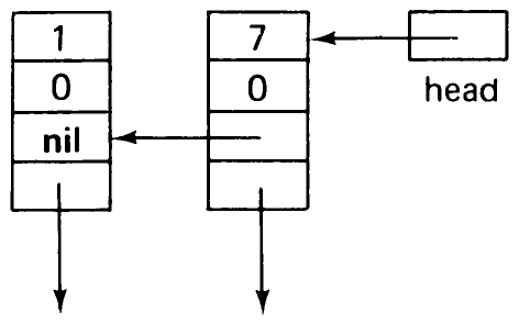
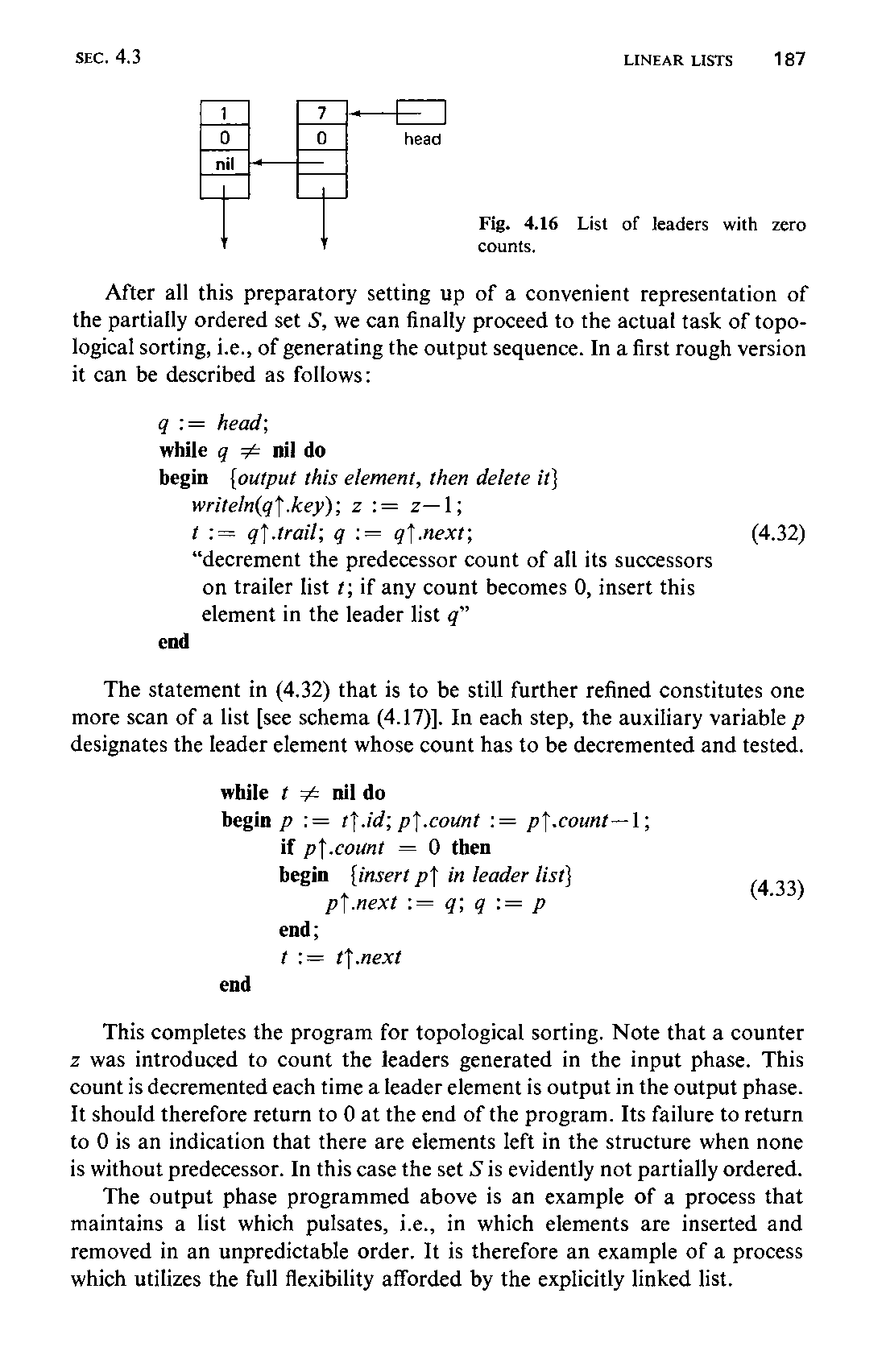
Referring to Fig. 4.15, we see that the next chain of leaders is replaced by the one of Fig. 4.16 in which the pointers not depicted are left unchanged.

186

187

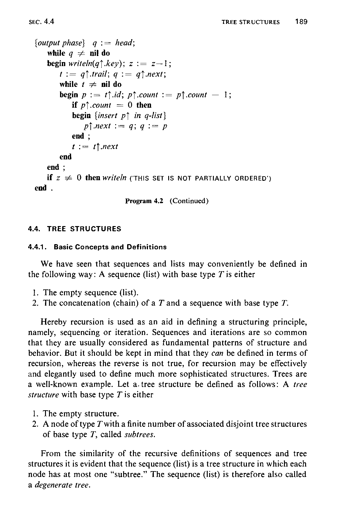
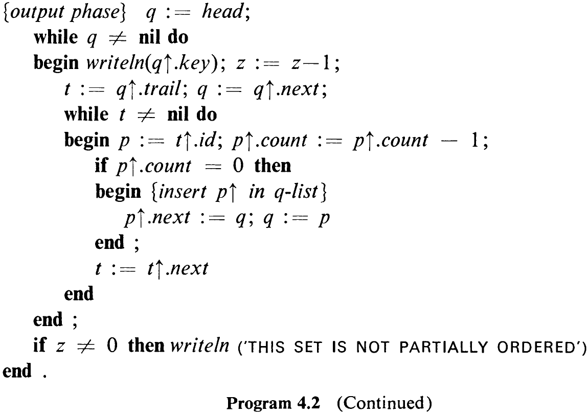
After all this preparatory setting up of a convenient representation of the partially ordered set $S$, we can finally proceed to the actual task of topological sorting, i.e., of generating the output sequence. In a first rough version it can be described as follows:

q := head;
while q ≠ nil do
begin {output this element, then delete it}
  writeln(q↑.key); z := z-1;
  t := q↑.trail; q := q↑.next;
  “decrement the predecessor count of all its successors
   on trailer list t; if any count becomes 0, insert this
   element in the leader list q”
end

The statement in (4.32) that is to be still further refined constitutes one more scan of a list [see schema (4.17)]. In each step, the auxiliary variable $p$ designates the leader element whose count has to be decremented and tested.

while t ≠ nil do
begin p := t↑.id; p↑.count := p↑.count-1;
      if p↑.count = 0 then
      begin {insert p↑ in leader list}
         p↑.next := q; q := p
      end;
      t := t↑.next
end

This completes the program for topological sorting. Note that a counter $z$ was introduced to count the leaders generated in the input phase. This count is decremented each time a leader element is output in the output phase. It should therefore return to 0 at the end of the program. Its failure to return to 0 is an indication that there are elements left in the structure when none is without predecessor. In this case the set $S$ is evidently not partially ordered.

The output phase programmed above is an example of a process that maintains a list which pulsates, i.e., in which elements are inserted and removed in an unpredictable order. It is therefore an example of a process which utilizes the full flexibility afforded by the explicitly linked list.