Tree Structures

4.4.1 Basic Concepts and Definitions

We have seen that sequences and lists may conveniently be defined in the following way: A sequence (list) with base type T is either

1. The empty sequence (list).

2. The concatenation (chain) of a T and a sequence with base type T.

Hereby recursion is used as an aid in defining a structuring principle, namely, sequencing or iteration. Sequences and iterations are so common that they are usually considered as fundamental patterns of structure and behavior. But it should be kept in mind that they can be defined in terms of recursion, whereas the reverse is not true, for recursion may be effectively and elegantly used to define much more sophisticated structures. Trees are a well-known example. Let a.tree structure be defined as follows: A tree structure with base type T is either

1. The empty structure.

2. Anode of type 7 with a finite number of associated disjoint tree structures of base type T, called subtrees.

From the similarity of the recursive definitions of sequences and tree structures it is evident that the sequence (list) is a tree structure in which each node has at most one “subtree.” The sequence (list) is therefore also called a degenerate tree.

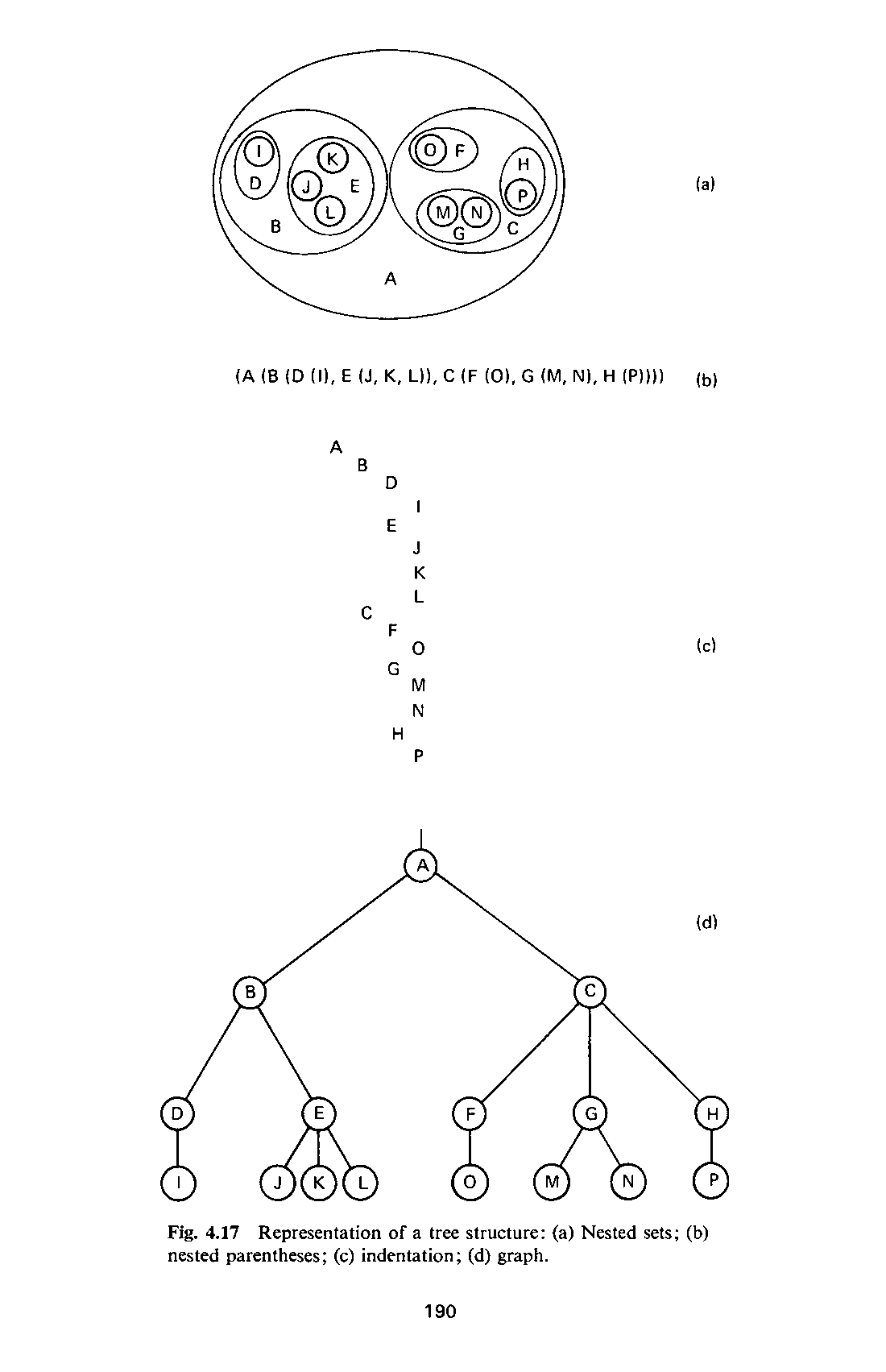
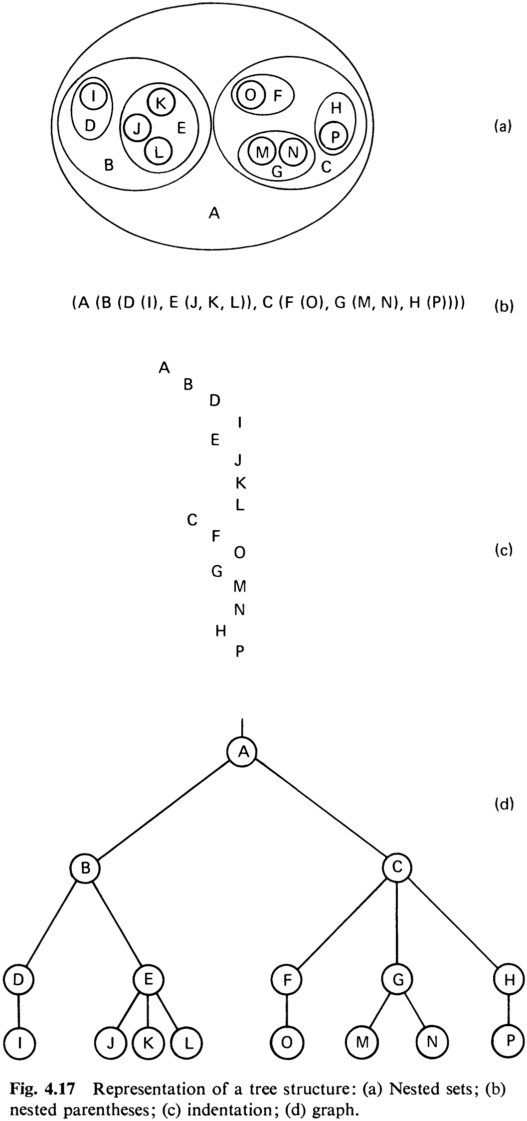
There are several ways to represent a tree structure. For example, let the base type T range over the letters; such a tree structure is shown in various ways in Fig. 4.17. These representations all show the same structure and are therefore equivalent. It is the graph structure that explicitly illustrates the branching relationships which, for obvious reasons, led to the generally used name “tree.” Strangely enough, it is customary to depict trees upside down, or—if one prefers to express this fact differently—to show the roots of trees. The latter formulation, however, is misleading, since the top node (A) is commonly called the root. Although we recognize that trees in nature are somewhat more complicated creations than our abstractions, henceforth we will call our tree structures simply trees.

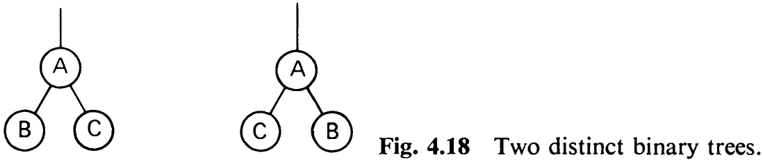
An ordered tree is a tree in which the branches of each node are ordered. Hence the two ordered trees in Fig. 4.18 are distinct, different objects. A node y which is directly below node x is called a (direct) descendant of x; if x is at Jevel i, then y is said to be a level i + 1. Inversely, node x is said to be the (direct) ancestor of y. The root of a tree is defined to be at level 1. The maximum level of any element of a tree is said to be its depth or height.

If an element has no descendants, it is called a terminal element or a leaf; and an element which is not terminal is an interior node. The number of (direct) descendants of an interior node is called its degree. The maximum degree over all nodes is the degree of the tree. The number of branches or edges which have to be traversed in order to proceed from the root to a node x is called the path length of x. The root has path length 1, its direct descendants have path length 2, etc. In general, a node at level i has path length i. The path length of a tree is defined as the sum of the path lengths of all its components. It is also called its internal path length. The internal path length of the tree shown in Fig. 4.17, for instance, is 52. Evidently, the average path length P, is

where n; is the number of nodes at level i. In order to define what is called the external path length, we extend the tree by a special node wherever a null subtree was present in the original tree. In doing so, we assume that all nodes are supposed to have the same degree, namely, the degree of the tree. Extending the tree in this way therefore amounts to filling up empty branches, whereby the special nodes, of course, have no further descendants. The tree of

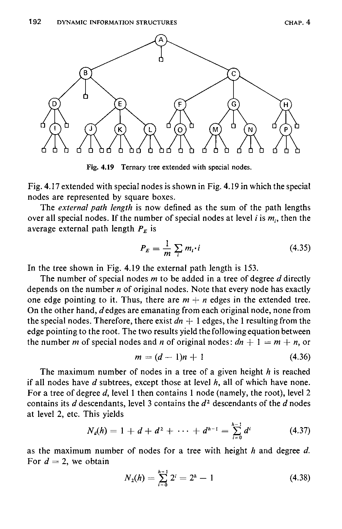
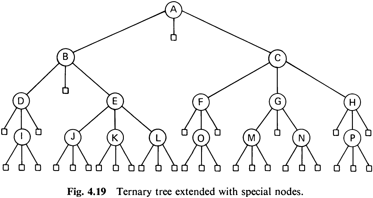
Fig. 4.17 extended with special nodes is shown in Fig. 4.19 in which the special nodes are represented by square boxes.

The external path length is now defined as the sum of the path lengths over all special nodes. If the number of special nodes at level i is m,, then the average external path length P;, is

In the tree shown in Fig. 4.19 the external path length is 153.

The number of special nodes m to be added in a tree of degree d directly depends on the number zx of original nodes. Note that every node has exactly one edge pointing to it. Thus, there are m + n edges in the extended tree. On the other hand, d edges are emanating from each original node, none from the special nodes. Therefore, there exist dn + 1 edges, the | resulting from the edge pointing to the root. The two results yield the following equation between the number m of special nodes and n of original nodes: dn + 1 = m+ n, or

The maximum number of nodes in a tree of a given height A is reached if all nodes have d subtrees, except those at level A, all of which have none. For a tree of degree d, level 1 then contains 1 node (namely, the root), level 2 contains its d descendants, level 3 contains the d* descendants of the d nodes at level 2, etc. This yields

as the maximum number of nodes for a tree with height A and degree d. For d = 2, we obtain

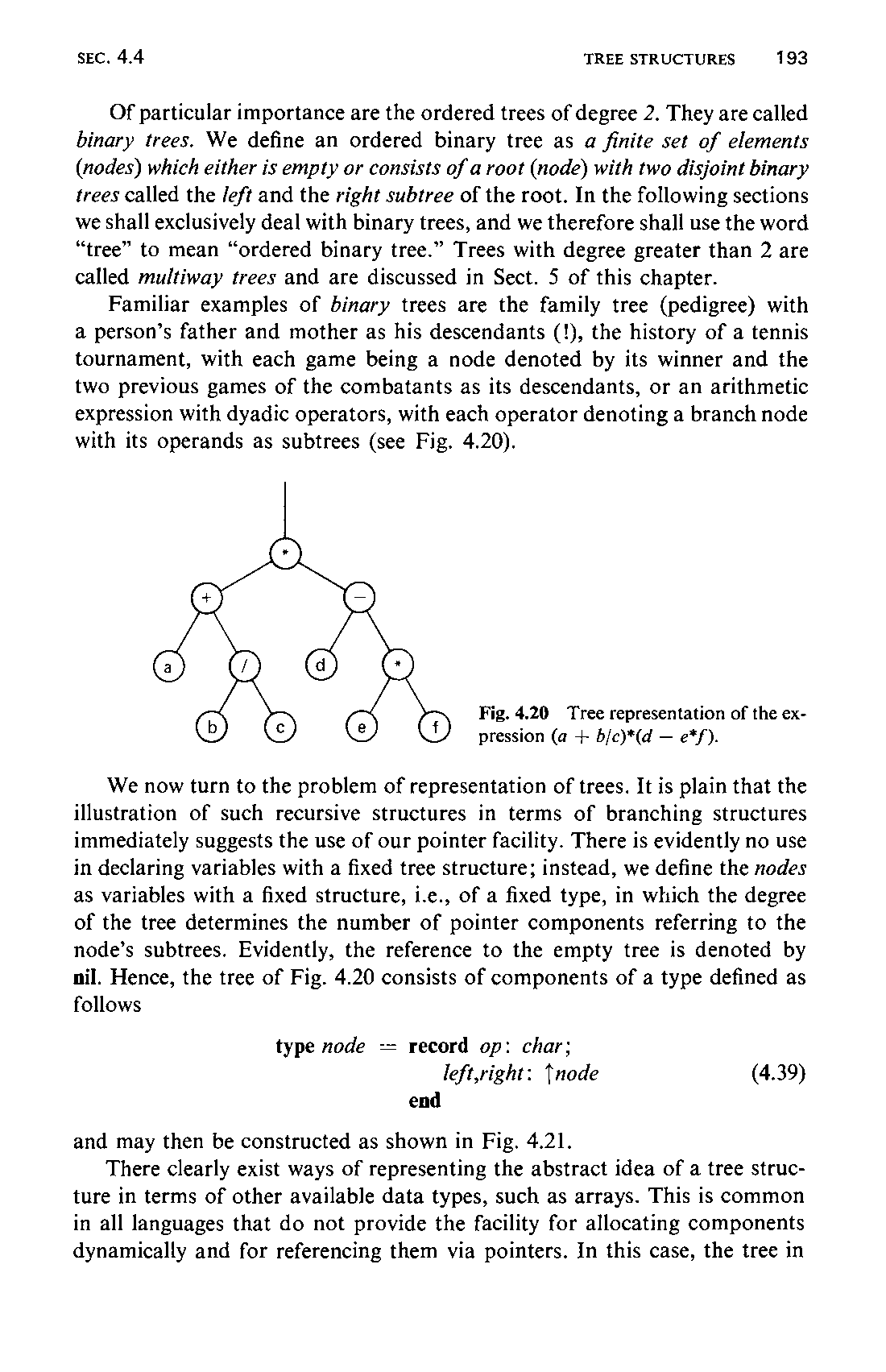
Of particular importance are the ordered trees of degree 2. They are called binary trees. We define an ordered binary tree as a finite set of elements (nodes) which either is empty or consists of a root (node) with two disjoint binary trees called the /eft and the right subtree of the root. In the following sections we shall exclusively deal with binary trees, and we therefore shall use the word “tree” to mean “ordered binary tree.” Trees with degree greater than 2 are called multiway trees and are discussed in Sect. 5 of this chapter.

Familiar examples of binary trees are the family tree (pedigree) with a person’s father and mother as his descendants (!), the history of a tennis tournament, with each game being a node denoted by its winner and the two previous games of the combatants as its descendants, or an arithmetic expression with dyadic operators, with each operator denoting a branch node with its operands as subtrees (see Fig. 4.20).

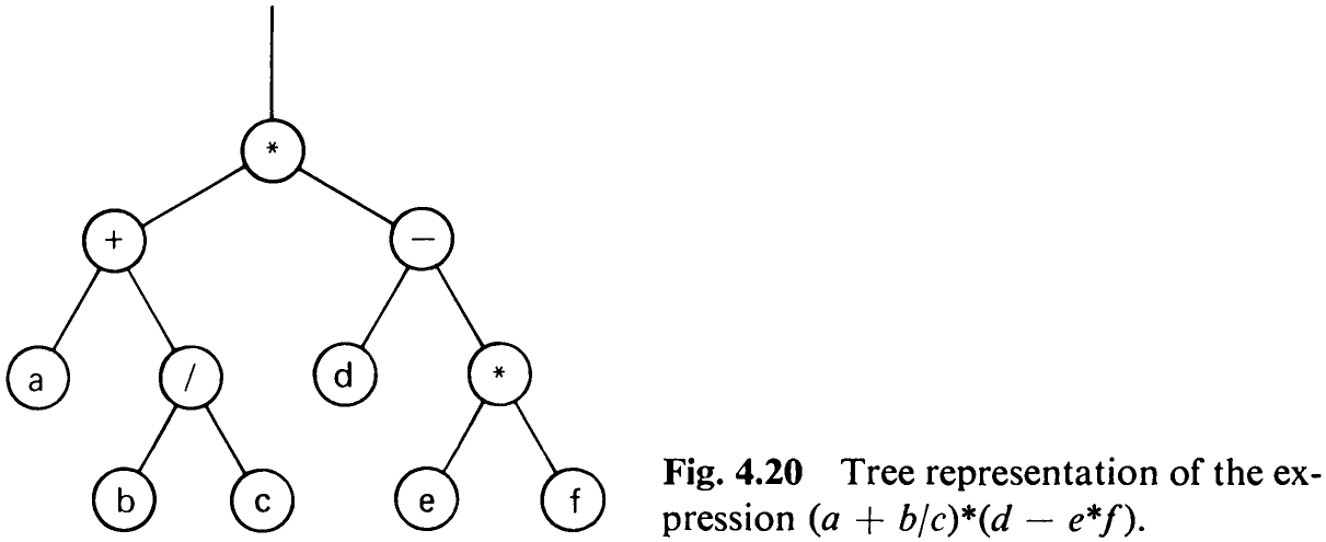
We now turn to the problem of representation of trees. It is plain that the illustration of such recursive structures in terms of branching structures immediately suggests the use of our pointer facility. There is evidently no use in declaring variables with a fixed tree structure; instead, we define the nodes as variables with a fixed structure, i.e., of a fixed type, in which the degree of the tree determines the number of pointer components referring to the node’s subtrees. Evidently, the reference to the empty tree is denoted by nil. Hence, the tree of Fig. 4.20 consists of components of a type defined as follows

and may then be constructed as shown in Fig. 4.21.

There clearly exist ways of representing the abstract idea of a tree structure in terms of other available data types, such as arrays. This is common in all languages that do not provide the facility for allocating components dynamically and for referencing them via pointers. In this case, the tree in

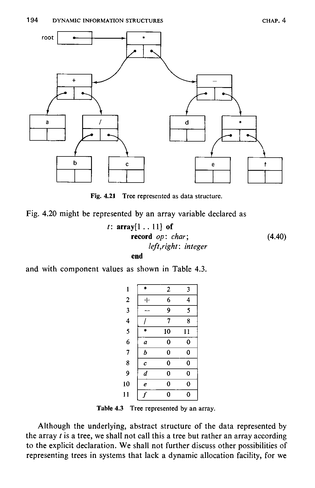
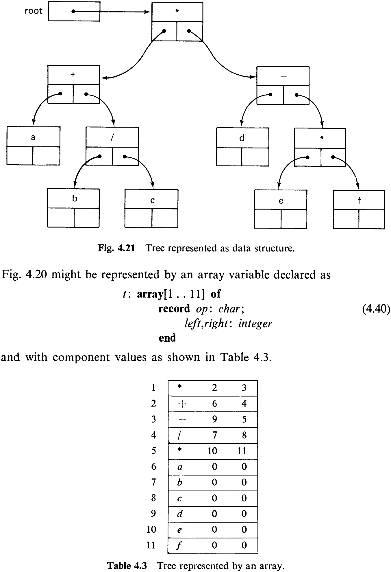
Although the underlying, abstract structure of the data represented by the array ¢ is a tree, we shall not call this a tree but rather an array according to the explicit declaration. We shall not further discuss other possibilities of representing trees in systems that lack a dynamic allocation facility, for we195 assume that programming systems and languages including this feature are or will become commonly available.

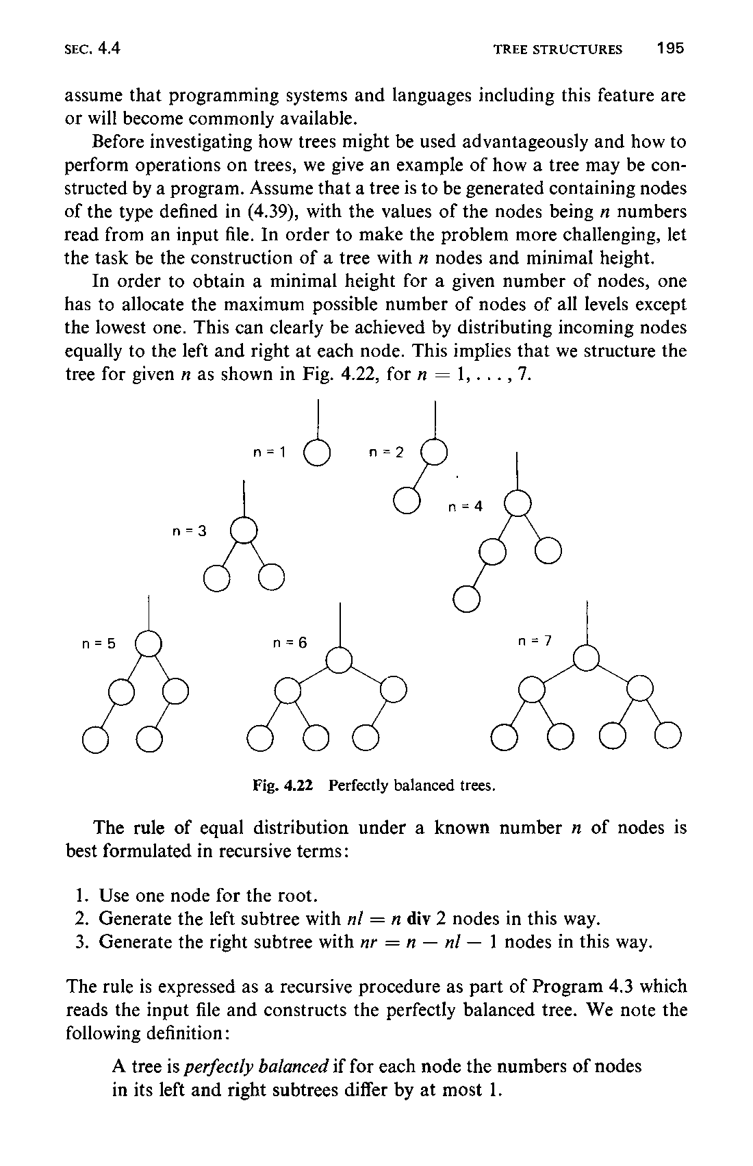
Before investigating how trees might be used advantageously and how to perform operations on trees, we give an example of how a tree may be constructed by a program. Assume that a tree is to be generated containing nodes of the type defined in (4.39), with the values of the nodes being n numbers read from an input file. In order to make the problem more challenging, let the task be the construction of a tree with m nodes and minimal height.

In order to obtain a minimal height for a given number of nodes, one has to allocate the maximum possible number of nodes of all levels except the lowest one. This can clearly be achieved by distributing incoming nodes equally to the left and right at each node. This impues shat we structure the tree for given n as shown in Fig. 4.22, forn = 1,.

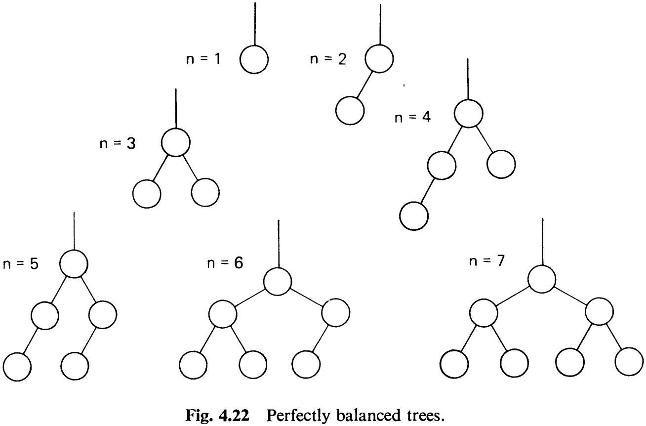
The rule of equal distribution under a known number x of nodes is best formulated in recursive terms:

1. Use one node for the root.

2. Generate the left subtree with nl = n div 2 nodes in this way.

3. Generate the right subtree with mr = n — nl — 1 nodes in this way.

The rule is expressed as a recursive procedure as part of Program 4.3 which reads the input file and constructs the perfectly balanced tree. We note the following definition:

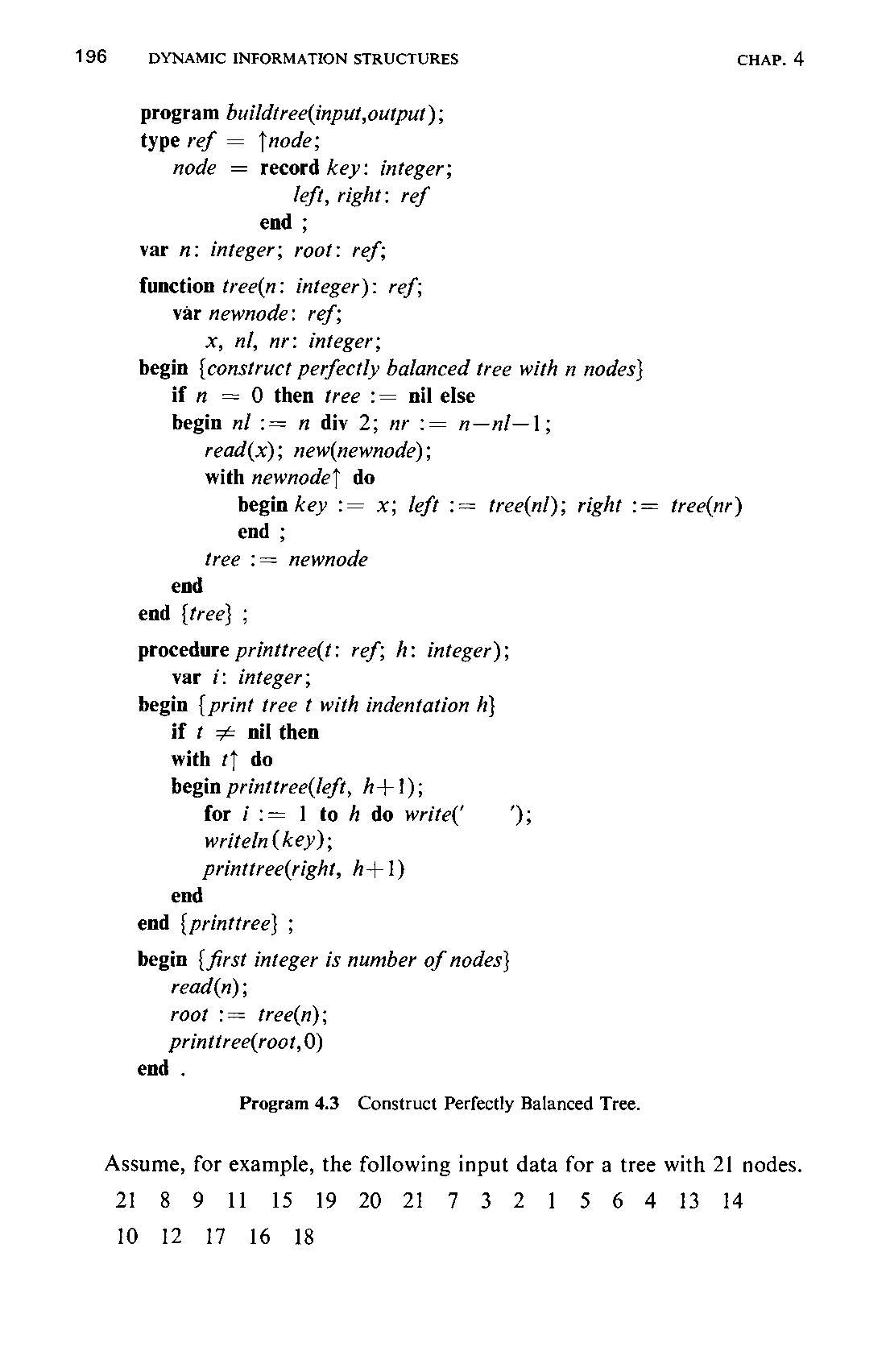
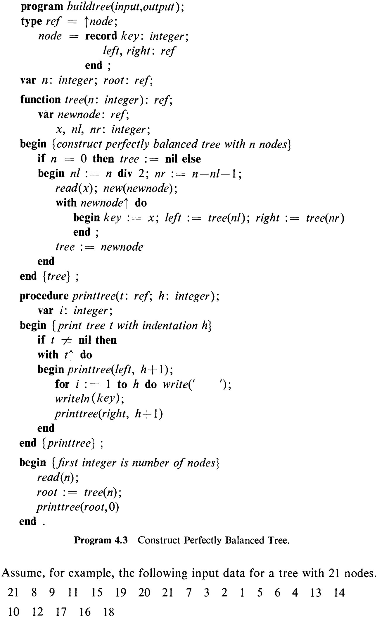
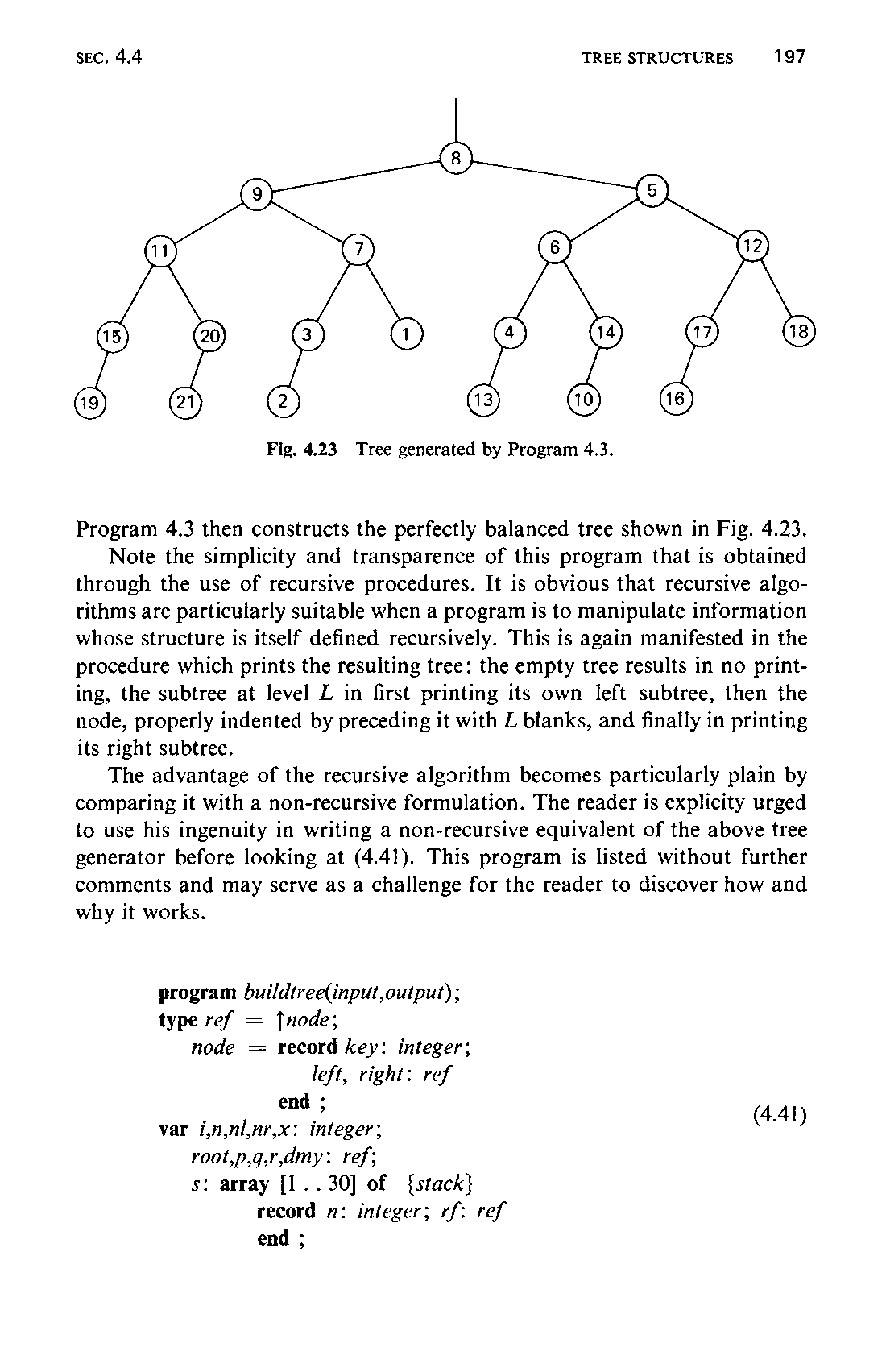
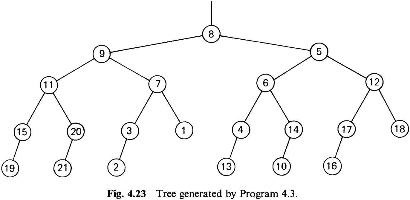
Program 4.3 then constructs the perfectly balanced tree shown in Fig. 4.23.

Note the simplicity and transparence of this program that is obtained through the use of recursive procedures. It is obvious that recursive algorithms are particularly suitable when a program is to manipulate information whose structure is itself defined recursively. This is again manifested in the procedure which prints the resulting tree: the empty tree results in no printing, the subtree at level L in first printing its own left subtree, then the node, properly indented by preceding it with Z blanks, and finally in printing its right subtree.

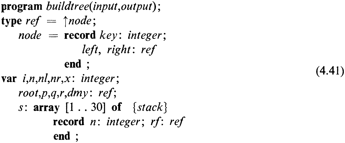
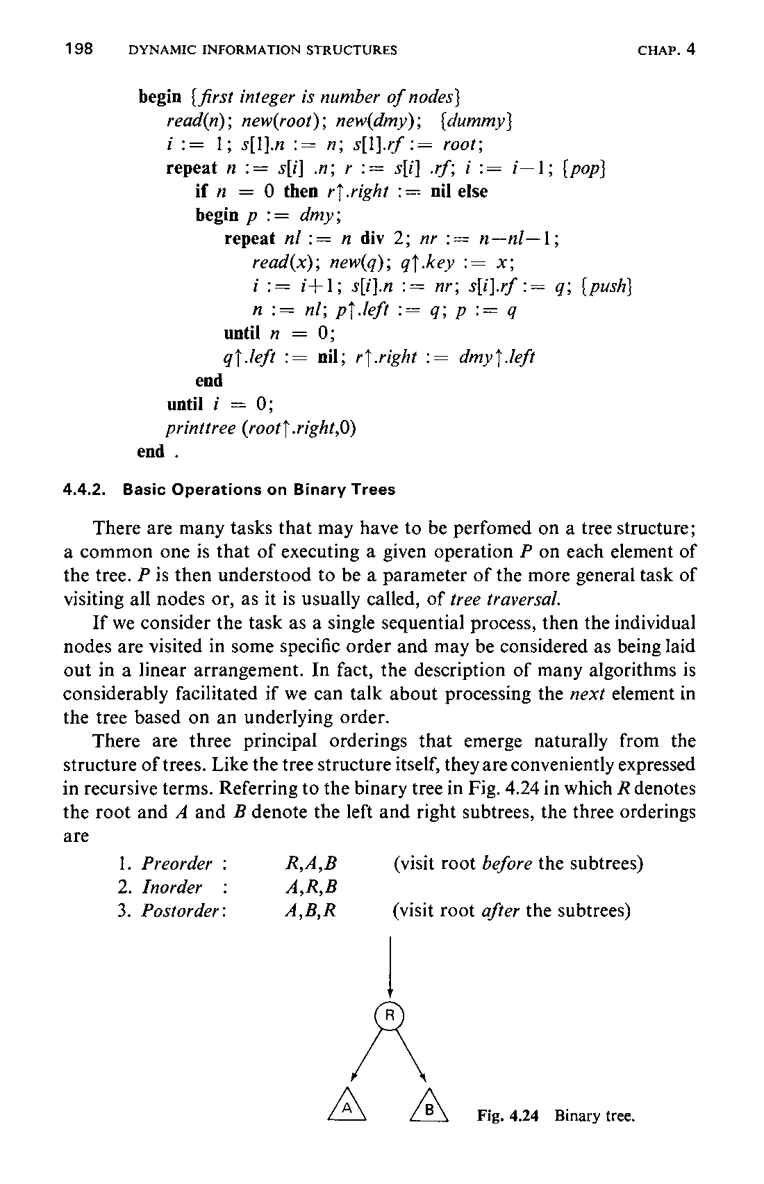
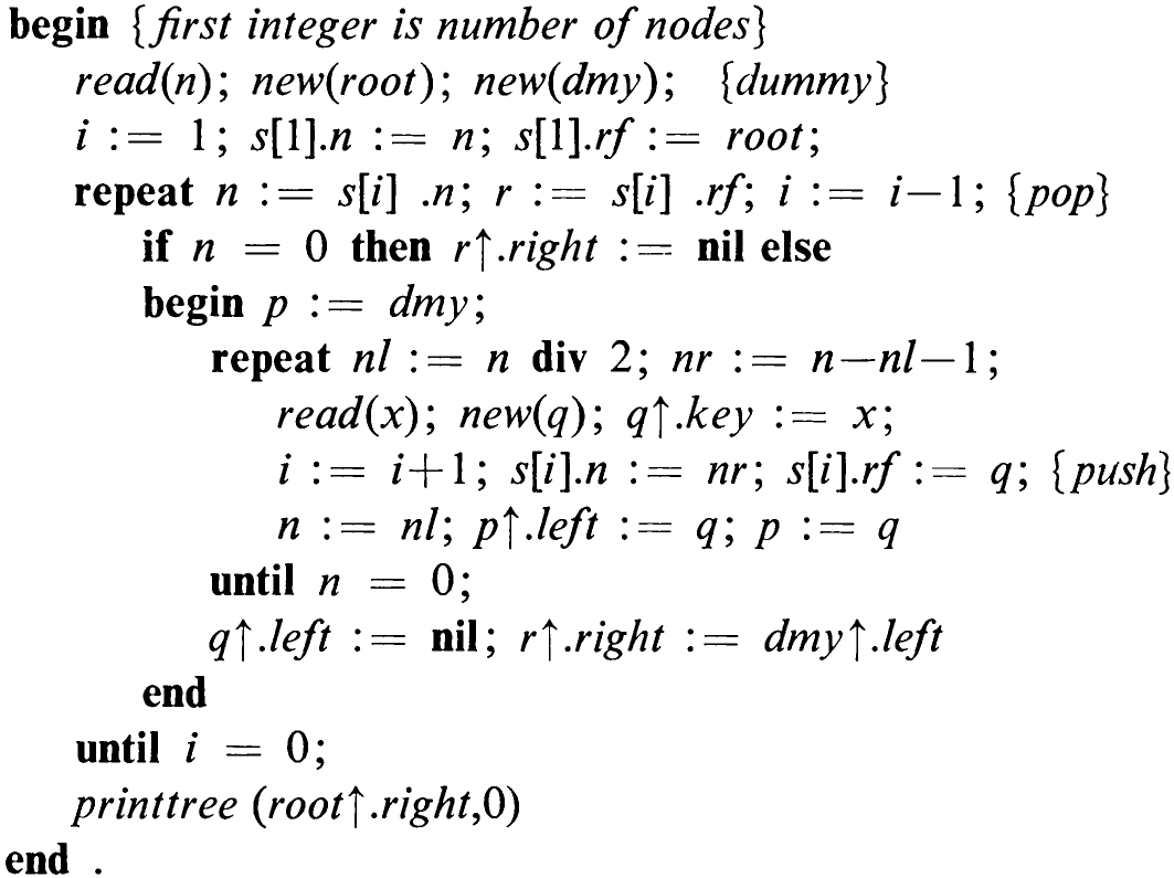
The advantage of the recursive algorithm becomes particularly plain by comparing it with a non-recursive formulation. The reader is explicity urged to use his ingenuity in writing a non-recursive equivalent of the above tree generator before looking at (4.41). This program is listed without further comments and may serve as a challenge for the reader to discover how and why it works.

4.4.2 Basic Operations on Binary Trees

There are many tasks that may have to be perfomed on a tree structure; a common one is that of executing a given operation P on each element of the tree. P is then understood to be a parameter of the more general task of visiting all nodes or, as it is usually called, of tree traversal.

If we consider the task as a single sequential process, then the individual nodes are visited in some specific order and may be considered as being laid out in a linear arrangement. In fact, the description of many algorithms is considerably facilitated if we can talk about processing the next element in the tree based on an underlying order.

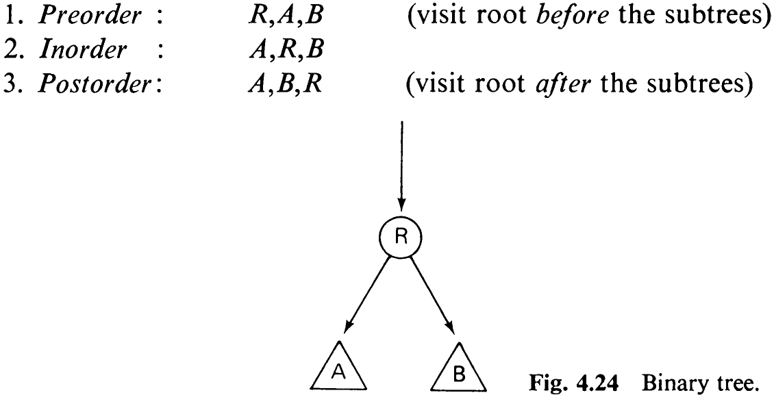
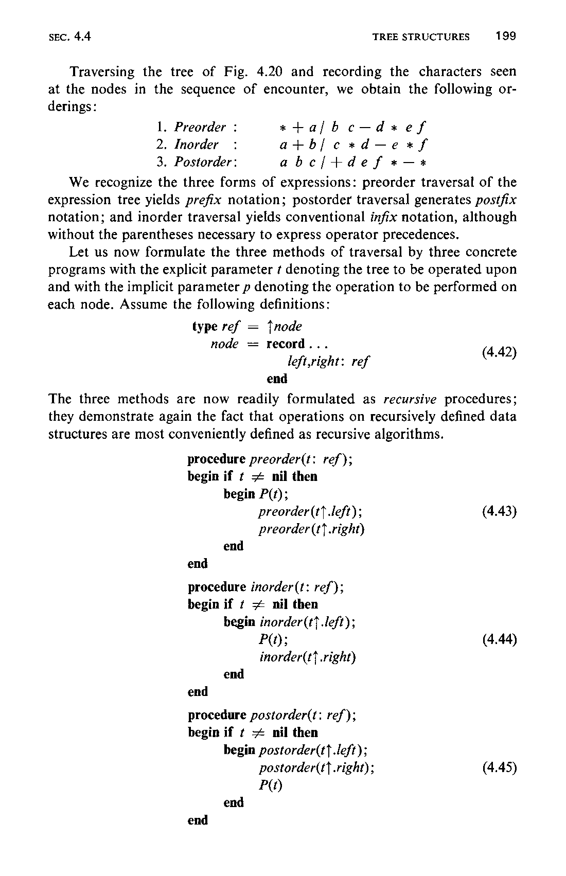
There are three principal orderings that emerge naturally from the structure of trees. Like the tree structure itself, they are conveniently expressed in recursive terms. Referring to the binary tree in Fig. 4.24 in which R denotes the root and A and B denote the left and right subtrees, the three orderings are

Traversing the tree of Fig. 4.20 and recording the characters seen at the nodes in the sequence of encounter, we obtain the following orderings:

We recognize the three forms of expressions: preorder traversal of the expression tree yields prefix notation; postorder traversal generates postfix notation; and inorder traversal yields conventional infix notation, although without the parentheses necessary to express operator precedences.

Let us now formulate the three methods of traversal by three concrete programs with the explicit parameter ¢ denoting the tree to be operated upon and with the implicit parameter p denoting the operation to be performed on each node. Assume the following definitions:

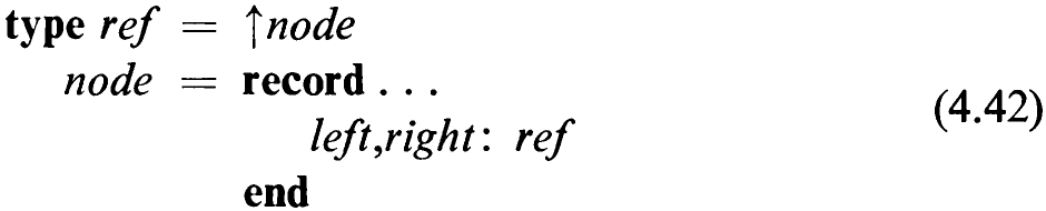
The three methods are now readily formulated as recursive procedures; they demonstrate again the fact that operations on recursively defined data structures are most conveniently defined as recursive algorithms.

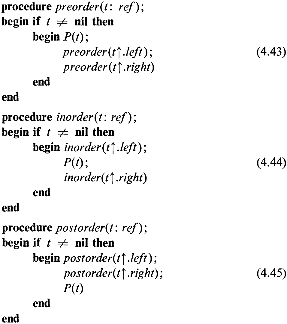
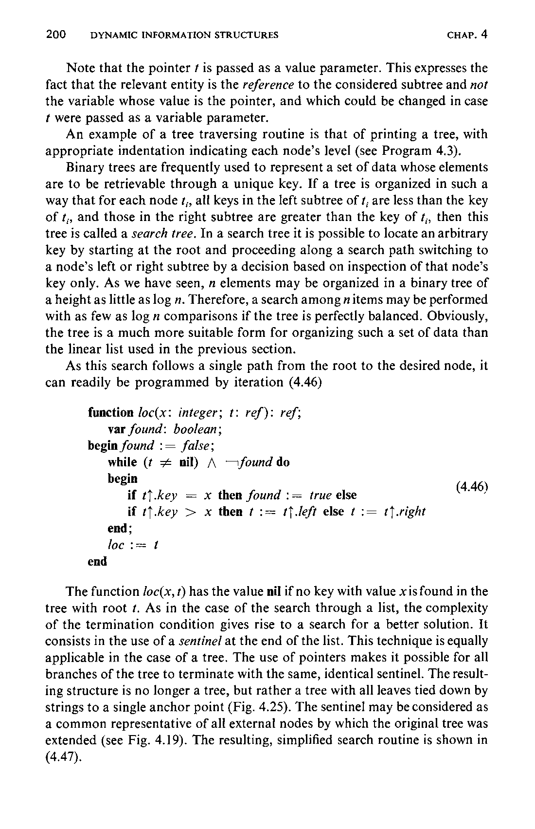
Note that the pointer ¢ is passed as a value parameter. This expresses the fact that the relevant entity is the reference to the considered subtree and not the variable whose value is the pointer, and which could be changed in case t were passed as a variable parameter.

An example of a tree traversing routine is that of printing a tree, with appropriate indentation indicating each node’s level (see Program 4.3).

Binary trees are frequently used to represent a set of data whose elements are to be retrievable through a unique key. If a tree is organized in such a way that for each node ¢,, all keys in the left subtree of t; are less than the key of t,, and those in the right subtree are greater than the key of ¢,, then this tree is called a search tree. In a search tree it is possible to locate an arbitrary key by starting at the root and proceeding along a search path switching to a node’s left or right subtree by a decision based on inspection of that node’s key only. As we have seen, n elements may be organized in a binary tree of a height as little as log n. Therefore, a search among nitems may be performed with as few as log n comparisons if the tree is perfectly balanced. Obviously, the tree is a much more suitable form for organizing such a set of data than the linear list used in the previous section.

As this search follows a single path from the root to the desired node, it can readily be programmed by iteration (4.46)

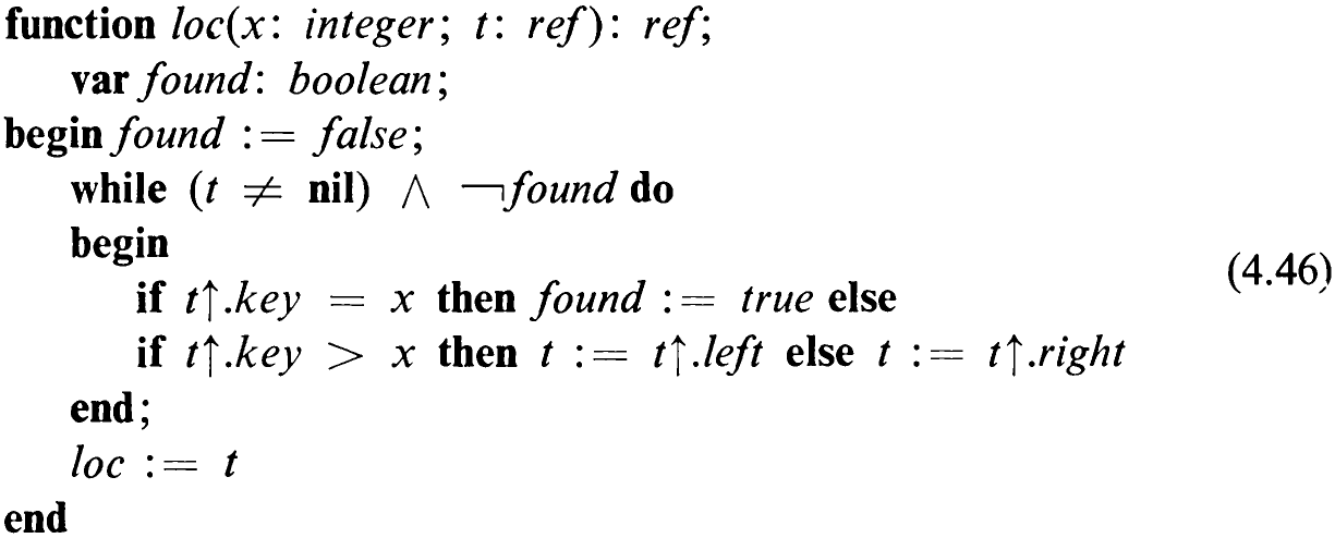
The function /oc(x, t) has the value nil if no key with value xis found in the tree with root ¢. As in the case of the search through a list, the complexity of the termination condition gives rise to a search for a better solution. It consists in the use of a sentinel at the end of the list. This technique is equally applicable in the case of a tree. The use of pointers makes it possible for all branches of the tree to terminate with the same, identical sentinel. The resulting structure is no longer a tree, but rather a tree with all leaves tied down by strings to a single anchor point (Fig. 4.25). The sentinel may be considered as a common representative of all external nodes by which the original tree was extended (see Fig. 4.19). The resulting, simplified search routine is shown in

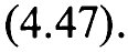
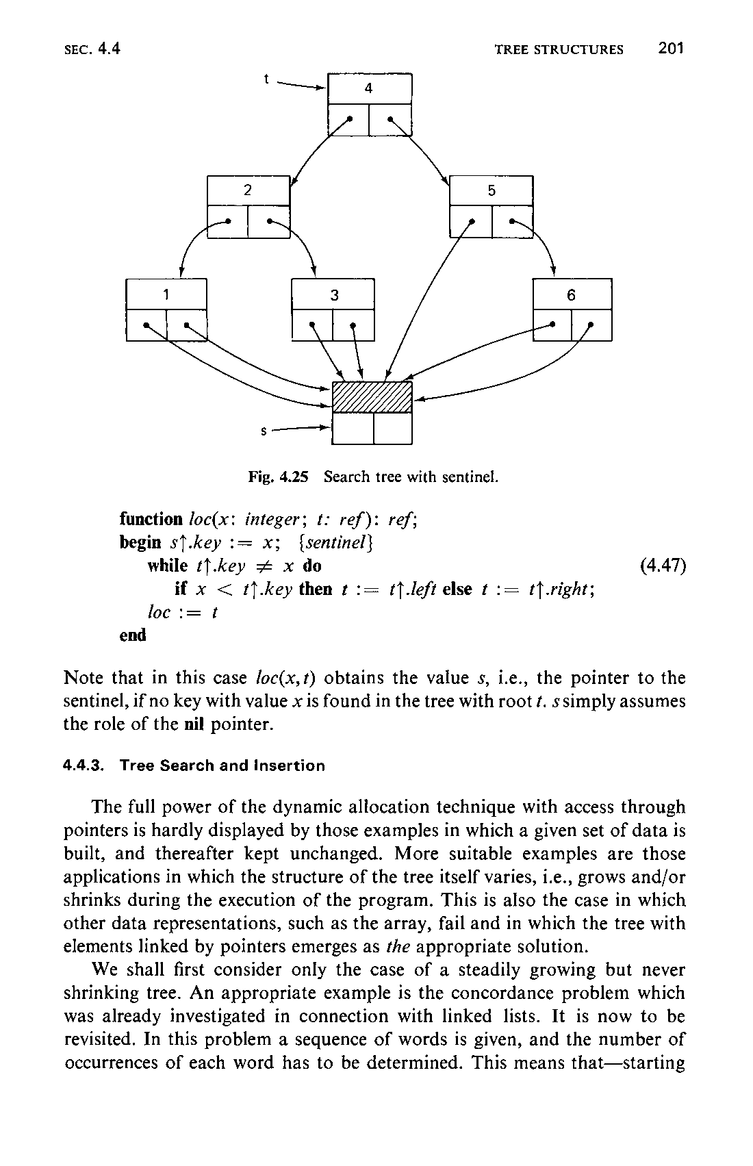
Note that in this case Joc(x,t) obtains the value s, i.e., the pointer to the sentinel, if no key with value x is found in the tree with root ¢. ssimply assumes the role of the nil pointer.

4.4.3 Tree Search and Insertion

The full power of the dynamic allocation technique with access through pointers is hardly displayed by those examples in which a given set of data is built, and thereafter kept unchanged. More suitable examples are those applications in which the structure of the tree itself varies, i.e., grows and/or shrinks during the execution of the program. This is also the case in which other data representations, such as the array, fail and in which the tree with elements linked by pointers emerges as the appropriate solution.

We shall first consider only the case of a steadily growing but never shrinking tree. An appropriate example is the concordance problem which was already investigated in connection with linked lists. It is now to be revisited. In this problem a sequence of words is given, and the number of occurrences of each word has to be determined. This means that—starting202 out with an empty tree—each word is searched in the tree. If it is found, its occurrence count is incremented; otherwise it is inserted as a new word (with a count initialized to 1). We call the underlying task tree search with insertion. The following data type definitions are assumed:

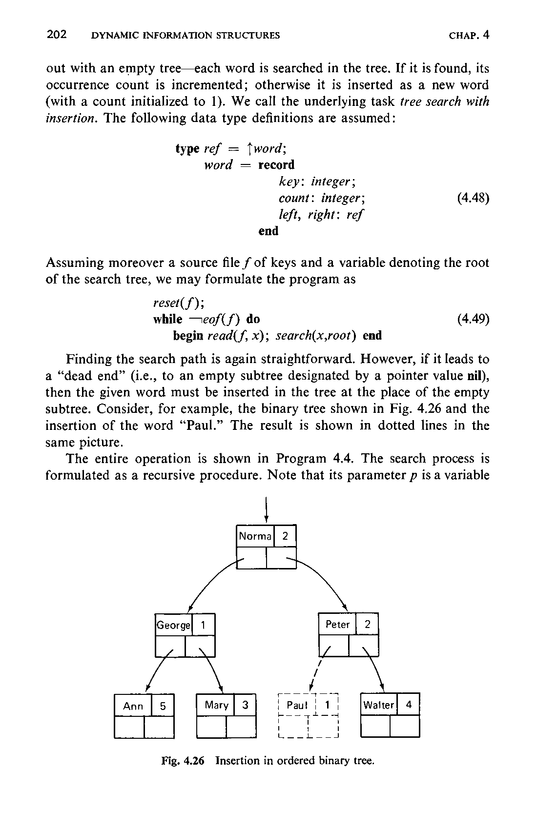
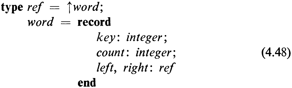
Assuming moreover a source file f of keys and a variable denoting the root of the search tree, we may formulate the program as

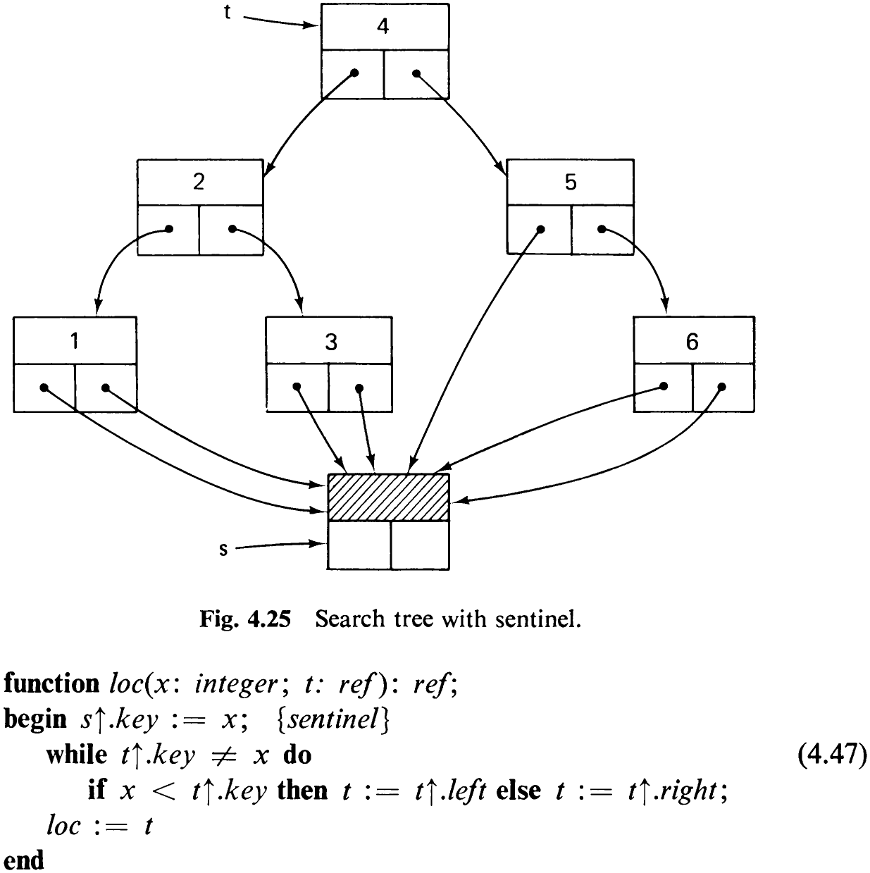
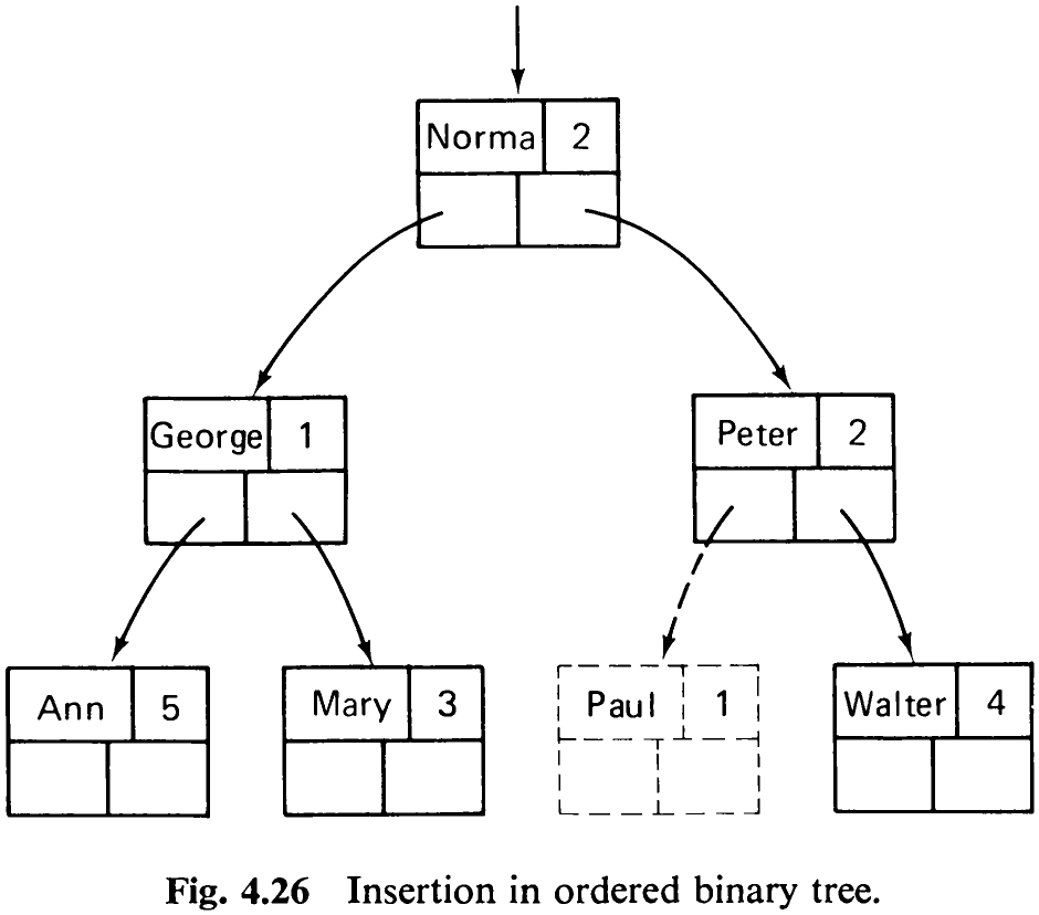
Finding the search path is again straightforward. However, if it leads to a “dead end” (i.e., to an empty subtree designated by a pointer value nil), then the given word must be inserted in the tree at the place of the empty subtree. Consider, for example, the binary tree shown in Fig. 4.26 and the insertion of the word “Paul.” The result is shown in dotted lines in the same picture.

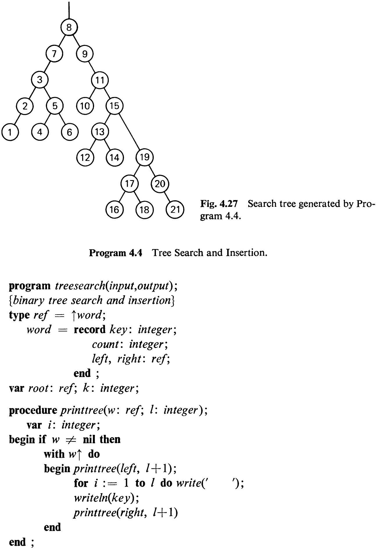
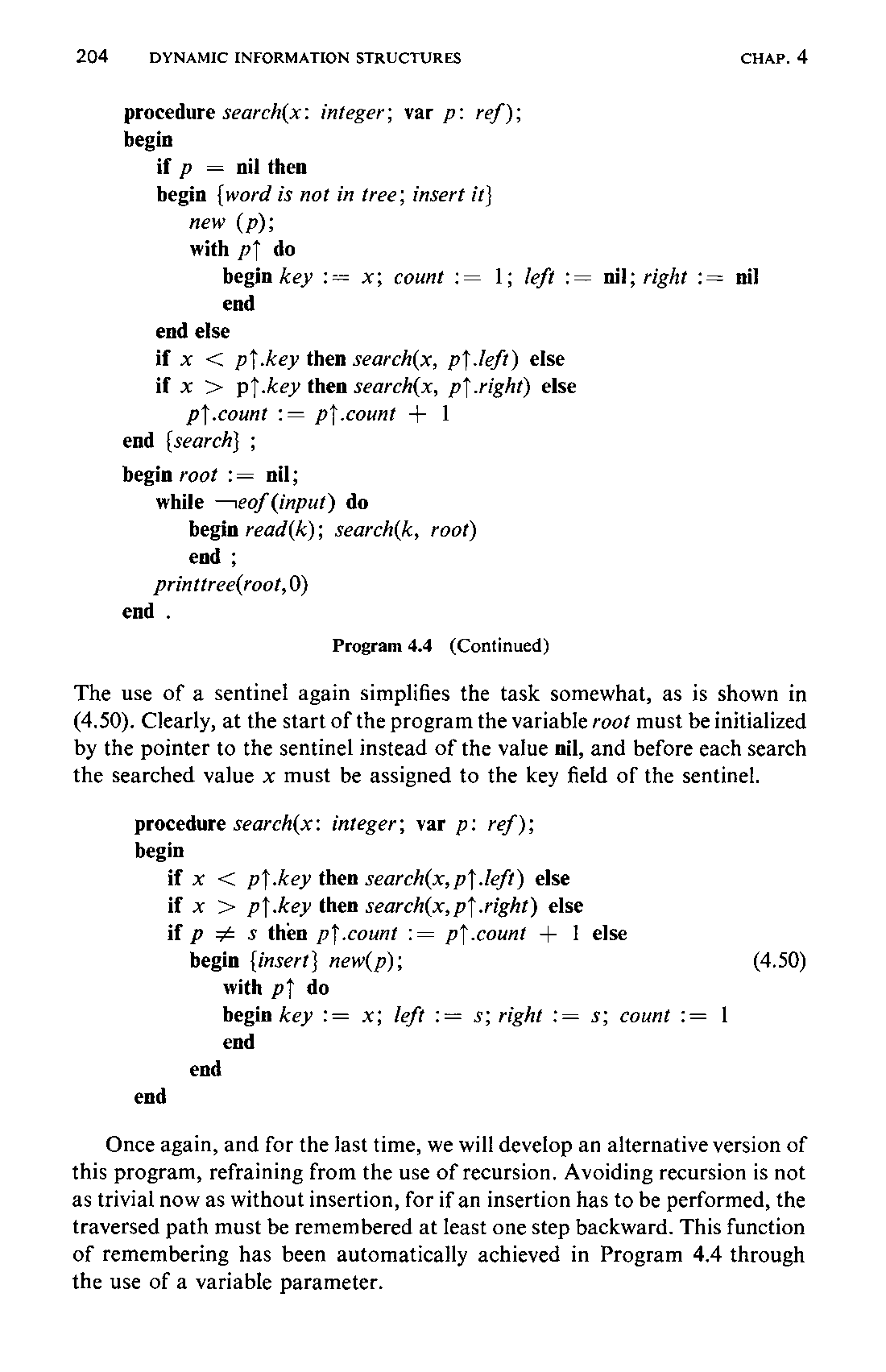
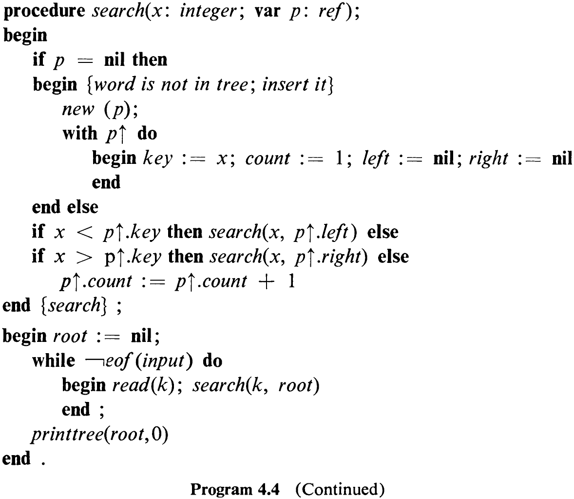
The entire operation is shown in Program 4.4. The search process is formulated as a recursive procedure. Note that its parameter p is a variable

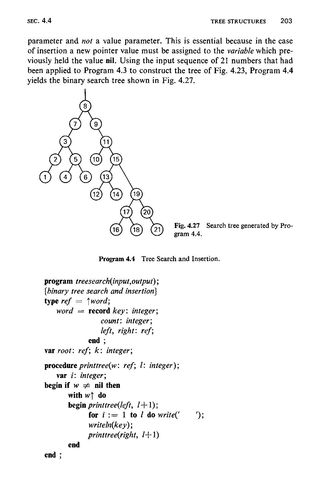
parameter and not a value parameter. This is essential because in the case of insertion a new pointer value must be assigned to the variable which previously held the value nil. Using the input sequence of 21 numbers that had been applied to Program 4.3 to construct the tree of Fig. 4.23, Program 4.4 yields the binary search tree shown in Fig. 4.27.

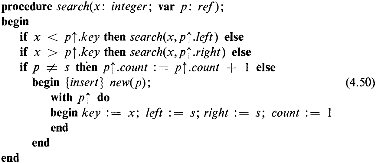
The use of a sentinel again simplifies the task somewhat, as is shown in (4.50). Clearly, at the start of the program the variable root must be initialized by the pointer to the sentinel instead of the value nil, and before each search the searched value x must be assigned to the key field of the sentinel.

Once again, and for the last time, we will develop an alternative version of this program, refraining from the use of recursion. Avoiding recursion is not as trivial now as without insertion, for if an insertion has to be performed, the traversed path must be remembered at least one step backward. This function of remembering has been automatically achieved in Program 4.4 through the use of a variable parameter.

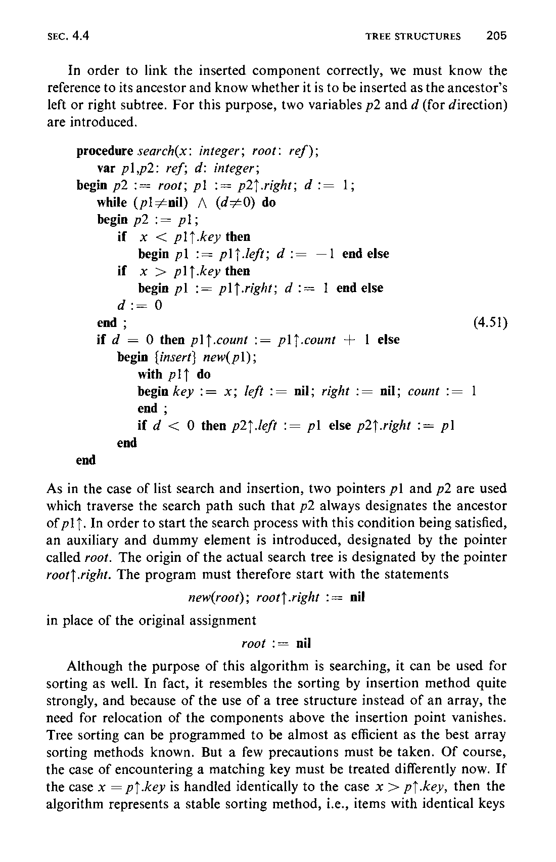
In order to link the inserted component correctly, we must know the reference to its ancestor and know whether it is to be inserted as the ancestor’s left or right subtree. For this purpose, two variables p2 and d (for direction) are introduced.

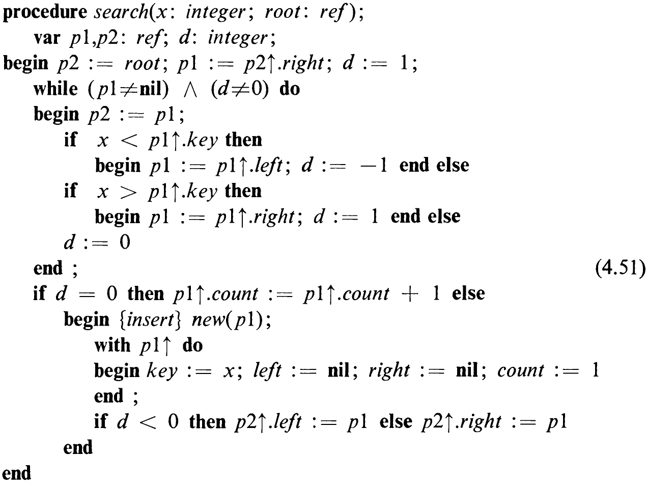
As in the case of list search and insertion, two pointers pl and p2 are used which traverse the search path such that p2 always designates the ancestor of plf. In order to start the search process with this condition being satisfied, an auxiliary and dummy element is introduced, designated by the pointer called root. The origin of the actual search tree is designated by the pointer root} .right. The program must therefore start with the statements

Although the purpose of this algorithm is searching, it can be used for sorting as well. In fact, it resembles the sorting by insertion method quite strongly, and because of the use of a tree structure instead of an array, the need for relocation of the components above the insertion point vanishes. Tree sorting can be programmed to be almost as efficient as the best array sorting methods known. But a few precautions must be taken. Of course, the case of encountering a matching key must be treated differently now. If the case x = p}.key is handled identically to the case x > p}.key, then the algorithm represents a stable sorting method, i.e., items with identical keys206 turn up in the same sequence when scanning the tree in normal order as when they were inserted.

In general, there are better ways to sort, but in applications in which searching and sorting are both needed, the tree search and insertion algorithm is strongly recommended. It is, in fact, very often applied in compilers and in data banks to organize the objects to be stored and retrieved. An appropriate example is the construction of a cross-reference index for a given text. Let us pursue this problem in detail.

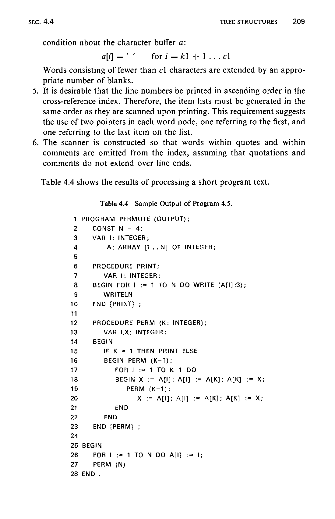
Our task is to construct a program that (while reading a text f and printing it after supplying consecutive line numbers) collects all words of this text, thereby retaining the numbers of the lines in which each word occurred. When this scan is terminated, a table is to be generated containing all collected words in alphabetical order with lists of their occurrences.

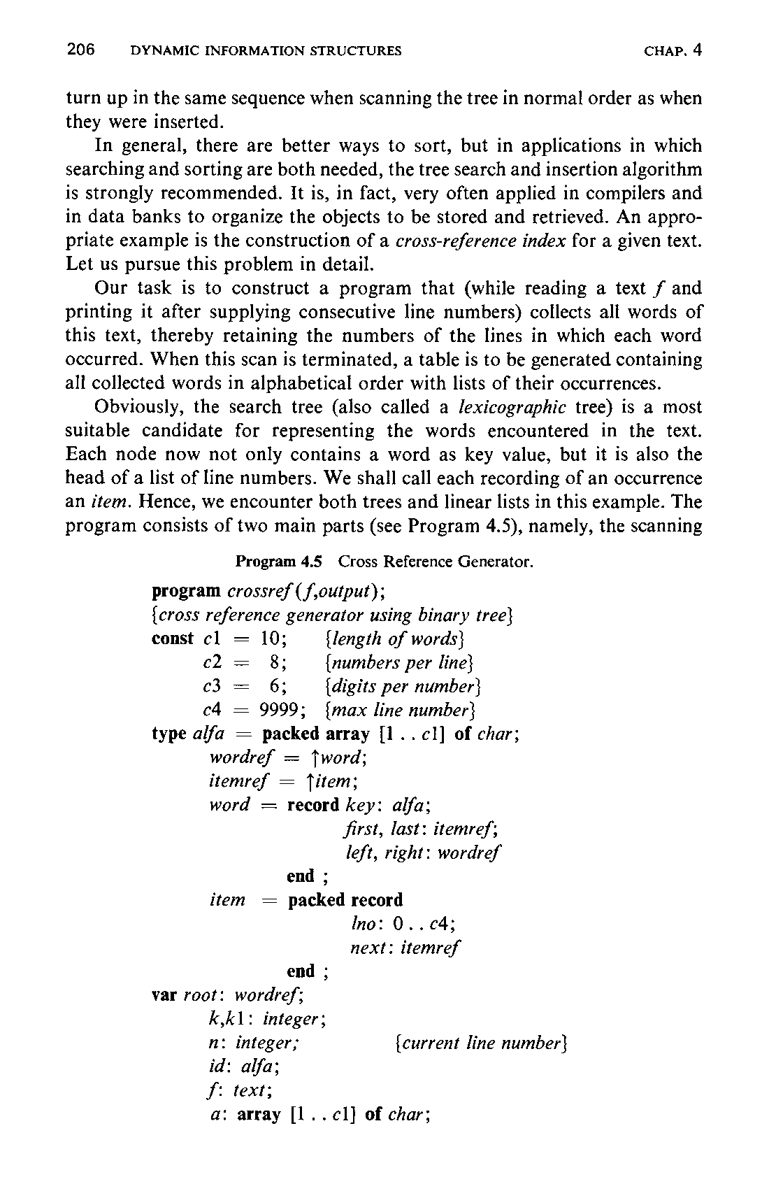
Obviously, the search tree (also called a lexicographic tree) is a most suitable candidate for representing the words encountered in the text. Each node now not only contains a word as key value, but it is also the head of a list of line numbers. We shall call each recording of an occurrence an item. Hence, we encounter both trees and linear lists in this example. The program consists of two main parts (see Program 4.5), namely, the scanning

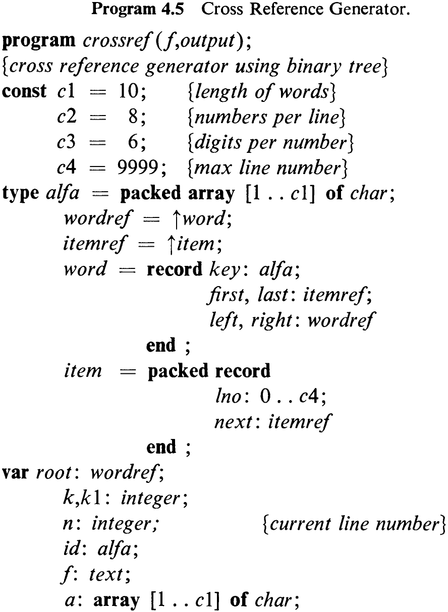
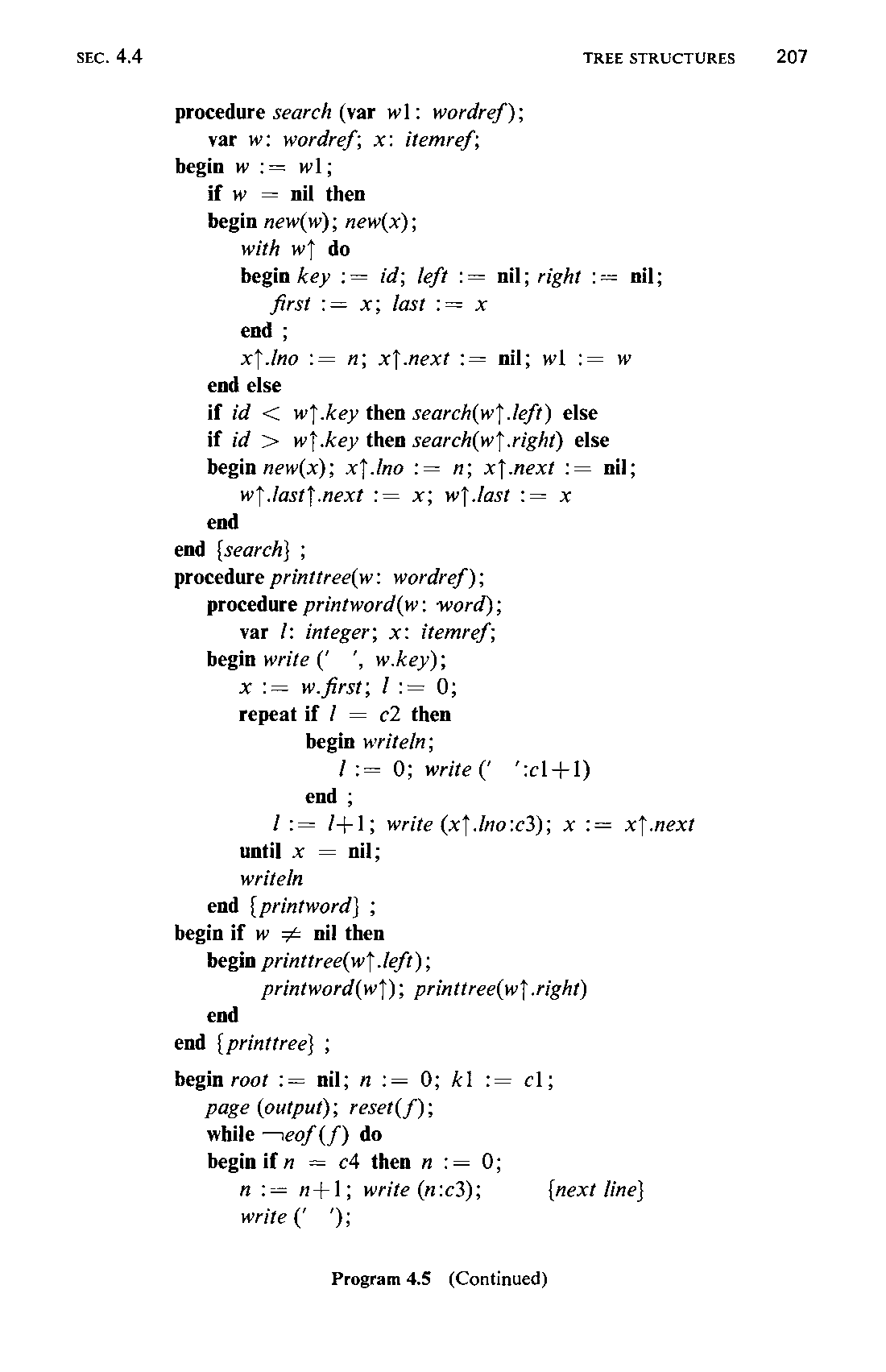
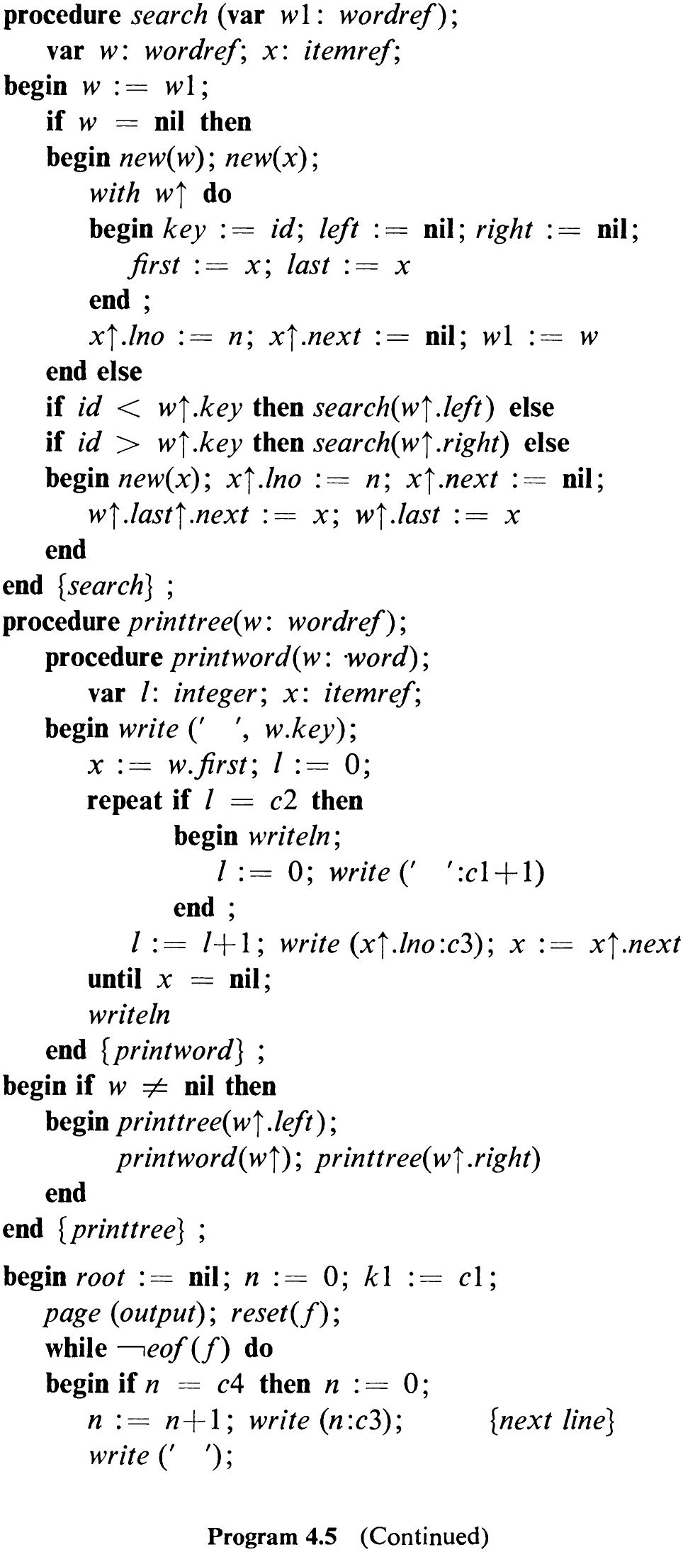
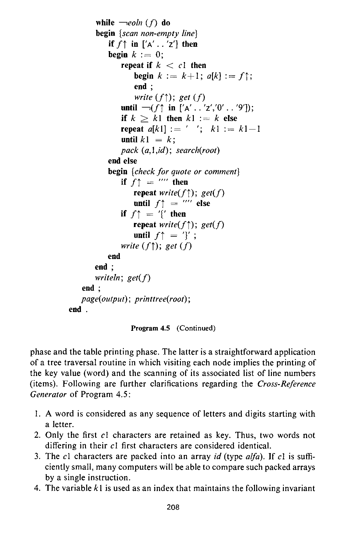
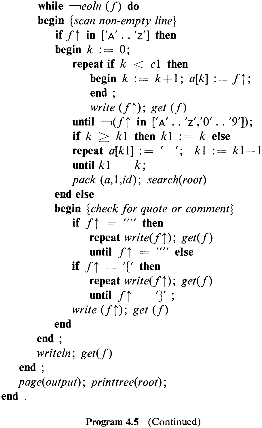
phase and the table printing phase. The latter is a straightforward application of a tree traversal routine in which visiting each node implies the printing of the key value (word) and the scanning of its associated list of line numbers (items). Following are further clarifications regarding the Cross-Reference Generator of Program 4.5:

1. A word is considered as any sequence of letters and digits starting with a letter.

2. Only the first cl characters are retained as key. Thus, two words not differing in their cl first characters are considered identical.

3. The cl characters are packed into an array id (type alfa). If cl is sufficiently small, many computers will be able to compare such packed arrays by a single instruction.

4. The variable k1 is used as an index that maintains the following invariant

Words consisting of fewer than cl characters are extended by an appropriate number of blanks.

5. It is desirable that the line numbers be printed in ascending order in the cross-reference index. Therefore, the item lists must be generated in the same order as they are scanned upon printing. This requirement suggests the use of two pointers in each word node, one referring to the first, and one referring to the last item on the list.

6. The scanner is constructed so that words within quotes and within comments are omitted from the index, assuming that quotations and comments do not extend over line ends.

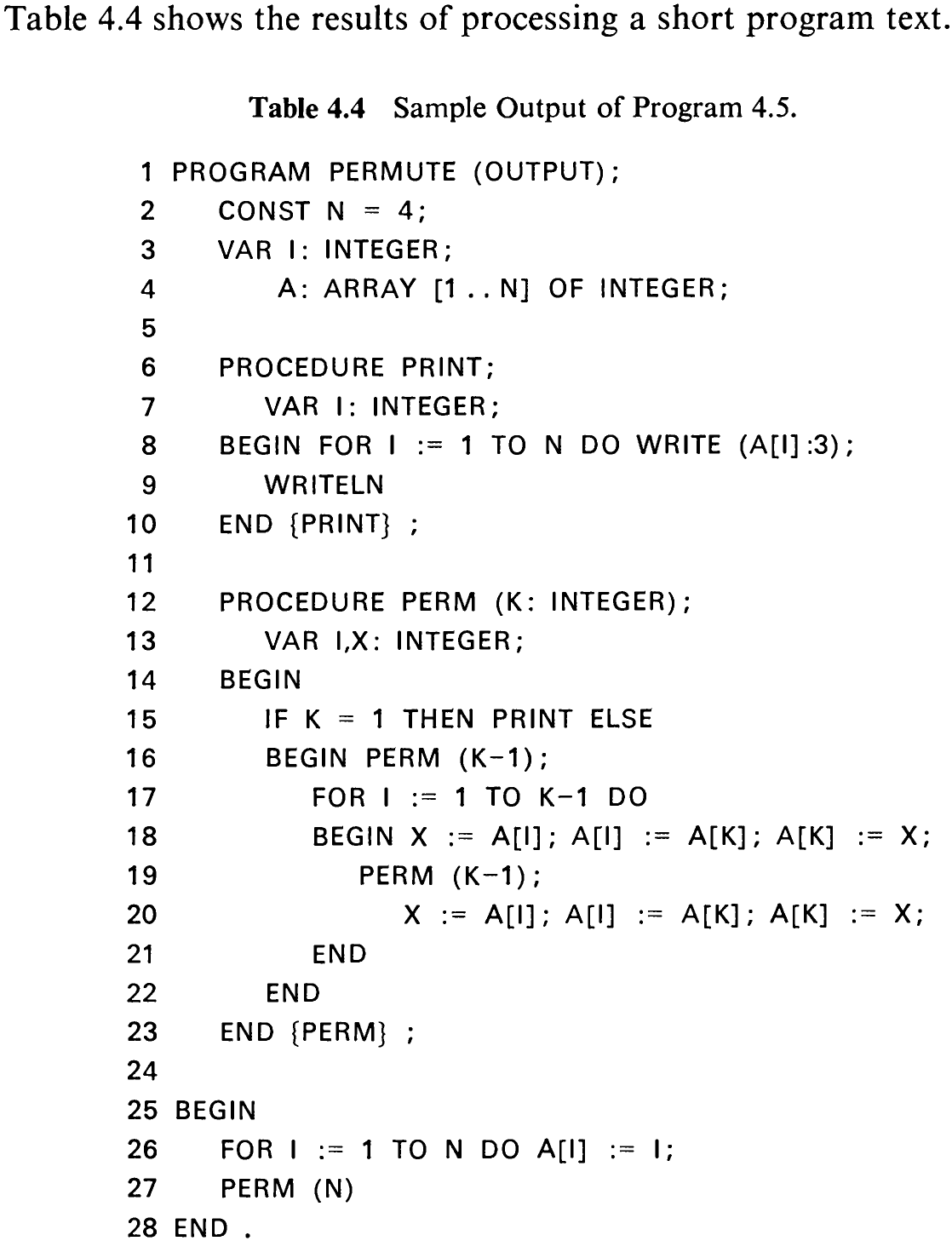
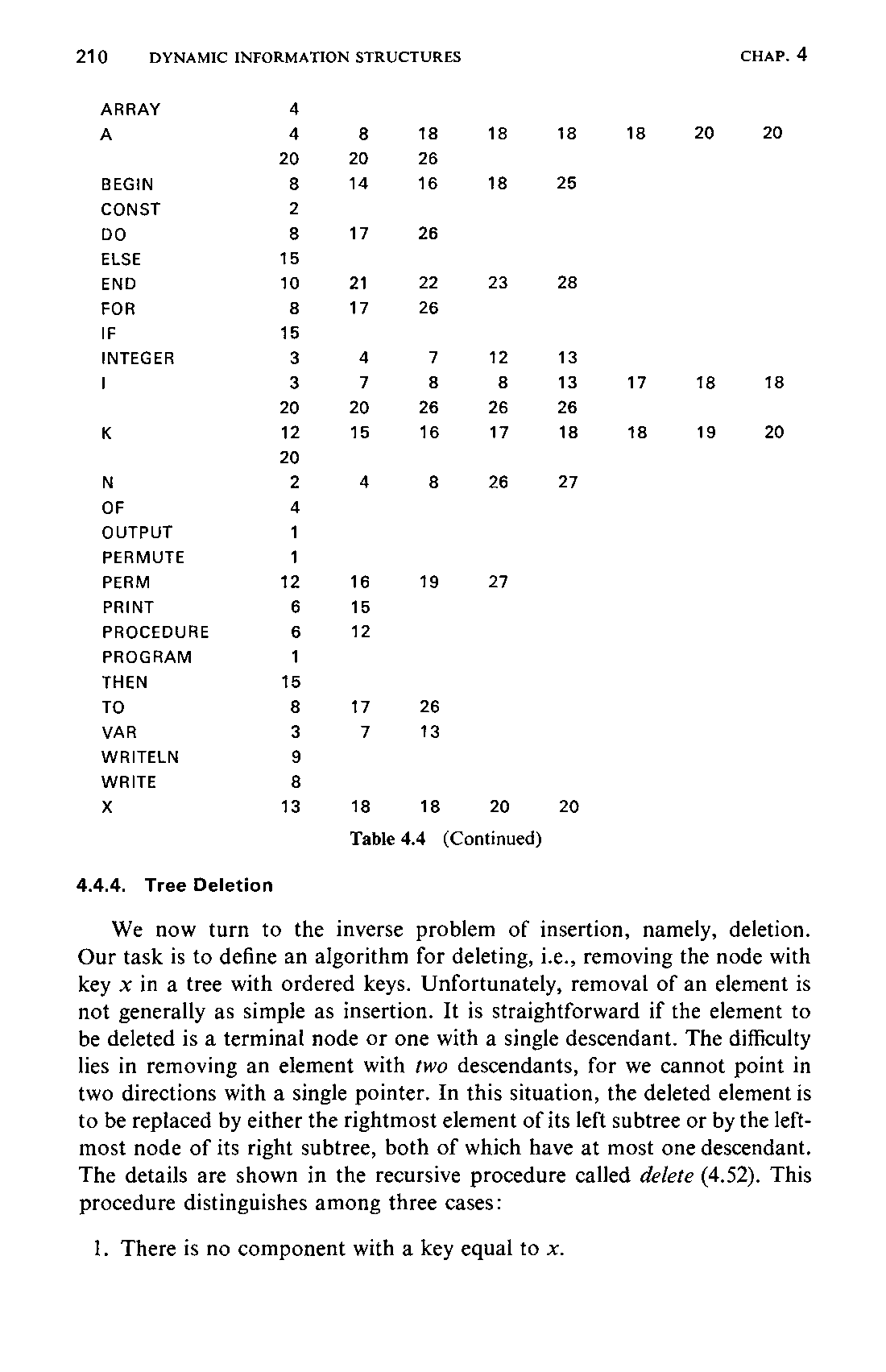
4.4.4 Tree Deletion

We now turn to the inverse problem of insertion, namely, deletion. Our task is to define an algorithm for deleting, i.e., removing the node with key x in a tree with ordered keys. Unfortunately, removal of an element is not generally as simple as insertion. It is straightforward if the element to be deleted is a terminal node or one with a single descendant. The difficulty lies in removing an element with two descendants, for we cannot point in two directions with a single pointer. In this situation, the deleted element is to be replaced by either the rightmost element of its left subtree or by the leftmost node of its right subtree, both of which have at most one descendant. The details are shown in the recursive procedure called delete (4.52). This procedure distinguishes among three cases:

1. There is no component with a key equal to x.

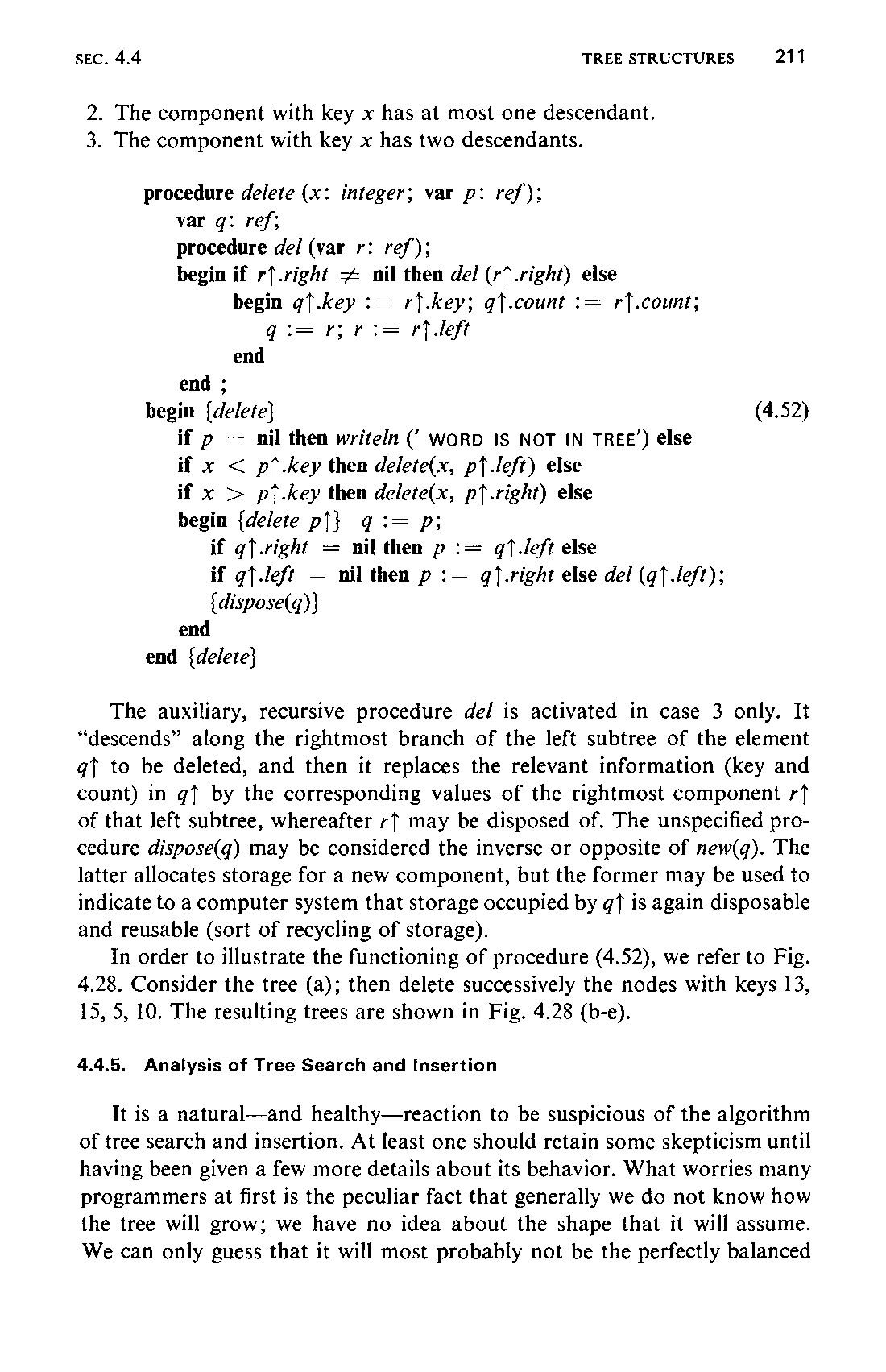
2. The component with key x has at most one descendant.

3. The component with key x has two descendants.

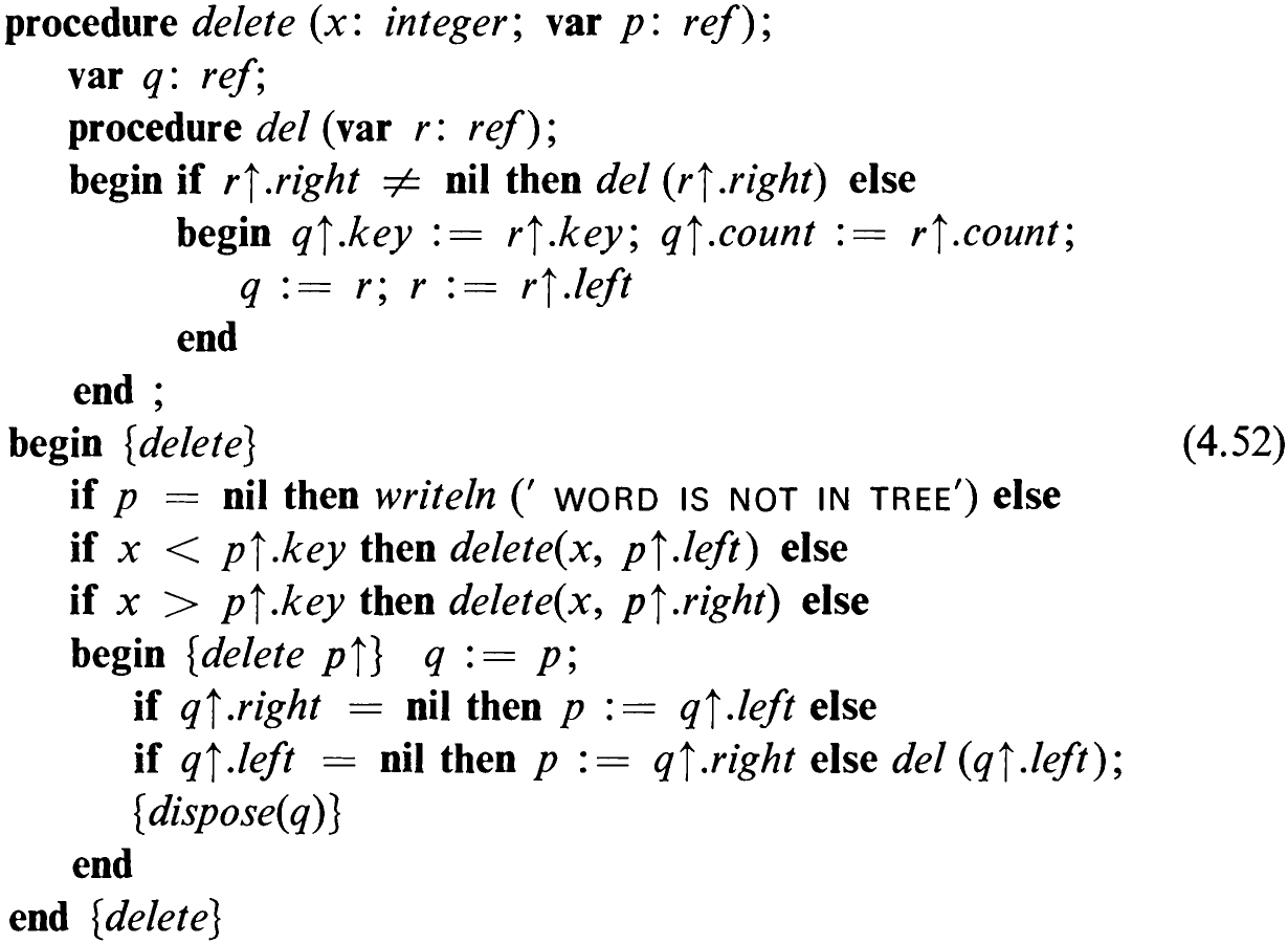
The auxiliary, recursive procedure de/ is activated in case 3 only. It “descends” along the rightmost branch of the left subtree of the element qt to be deleted, and then it replaces the relevant information (key and count) in qf by the corresponding values of the rightmost component rt of that left subtree, whereafter r} may be disposed of. The unspecified procedure dispose(q) may be considered the inverse or opposite of new(q). The latter allocates storage for a new component, but the former may be used to indicate to a computer system that storage occupied by gq? is again disposable and reusable (sort of recycling of storage).

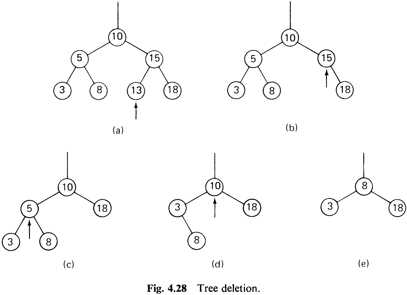
In order to illustrate the functioning of procedure (4.52), we refer to Fig. 4.28. Consider the tree (a); then delete successively the nodes with keys 13, 15, 5, 10. The resulting trees are shown in Fig. 4.28 (b-e).

4.4.5 Analysis of Tree Search and Insertion

It is a natural—and healthy—reaction to be suspicious of the algorithm of tree search and insertion. At least one should retain some skepticism until having been given a few more details about its behavior. What worries many programmers at first is the peculiar fact that generally we do not know how the tree will grow; we have no idea about the shape that it will assume. We can only guess that it will most probably not be the perfectly balanced

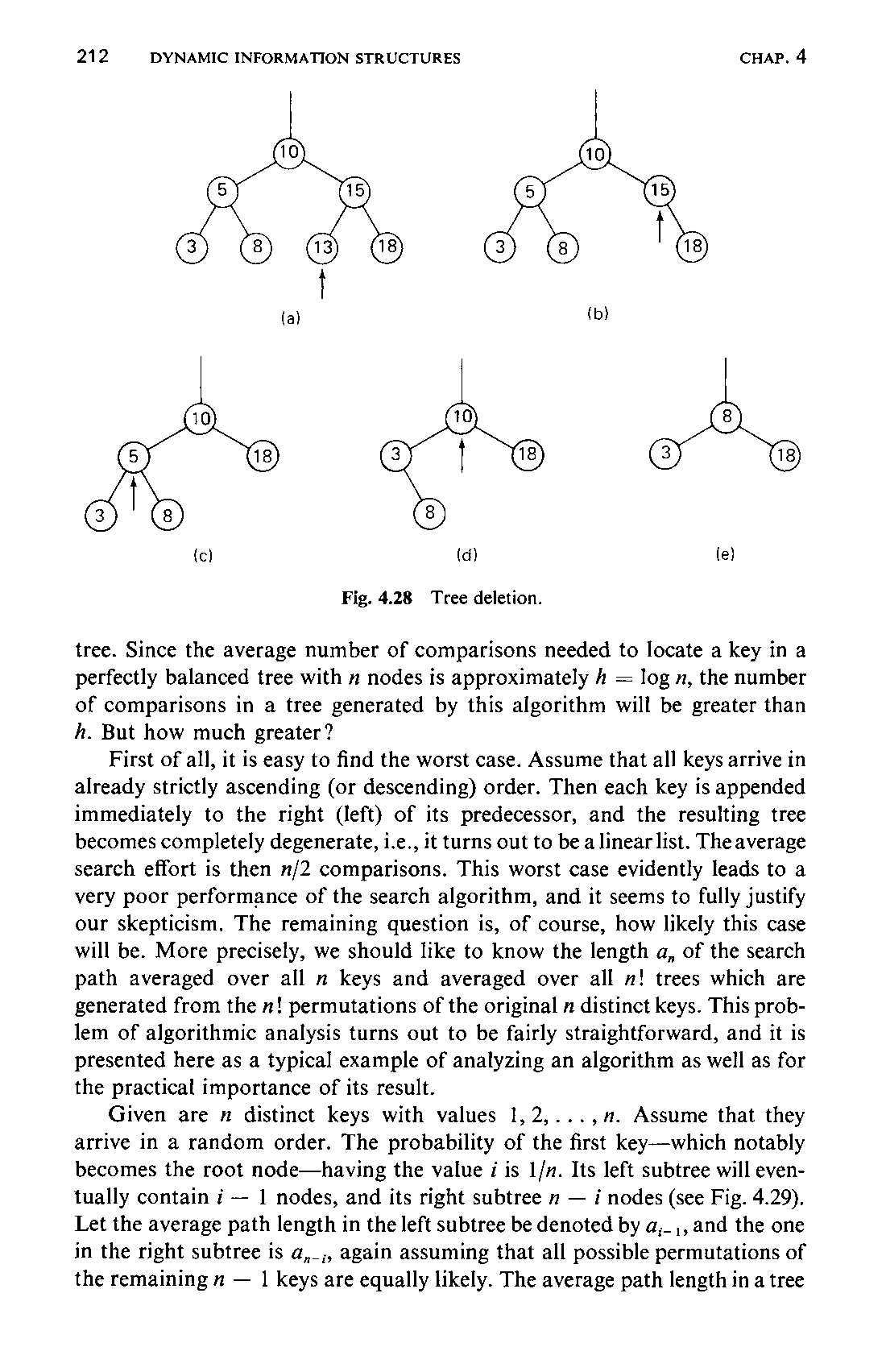
tree. Since the average number of comparisons needed to locate a key in a perfectly balanced tree with n nodes is approximately 4 = log n, the number of comparisons in a tree generated by this algorithm will be greater than h. But how much greater?

First of all, it is easy to find the worst case. Assume that all keys arrive in already strictly ascending (or descending) order. Then each key is appended immediately to the right (left) of its predecessor, and the resulting tree becomes completely degenerate, i.e., it turns out to be a linear list. The average search effort is then n/2 comparisons. This worst case evidently leads to a very poor performance of the search algorithm, and it seems to fully justify our skepticism. The remaining question is, of course, how likely this case will be. More precisely, we should like to know the length a, of the search path averaged over all n keys and averaged over all m! trees which are generated from the n! permutations of the original n distinct keys. This problem of algorithmic analysis turns out to be fairly straightforward, and it is presented here as a typical example of analyzing an algorithm as well as for the practical importance of its result.

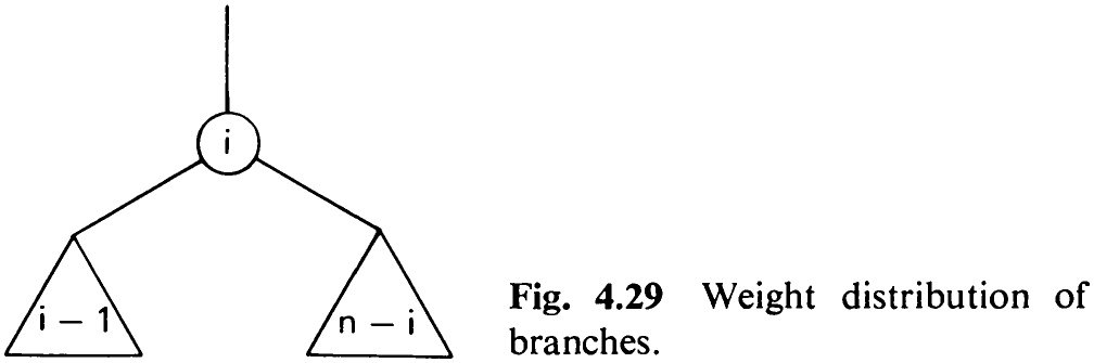
Given are n distinct keys with values 1, 2,...,2. Assume that they arrive in a random order. The probability of the first key—which notably becomes the root node—having the value i is 1/n. Its left subtree will eventually contain i — 1 nodes, and its right subtree n — i nodes (see Fig. 4.29). Let the average path length in the left subtree be denoted by a;_,, and the one in the right subtree is a,_,, again assuming that all possible permutations of the remaining n — | keys are equally likely. The average path length in a tree

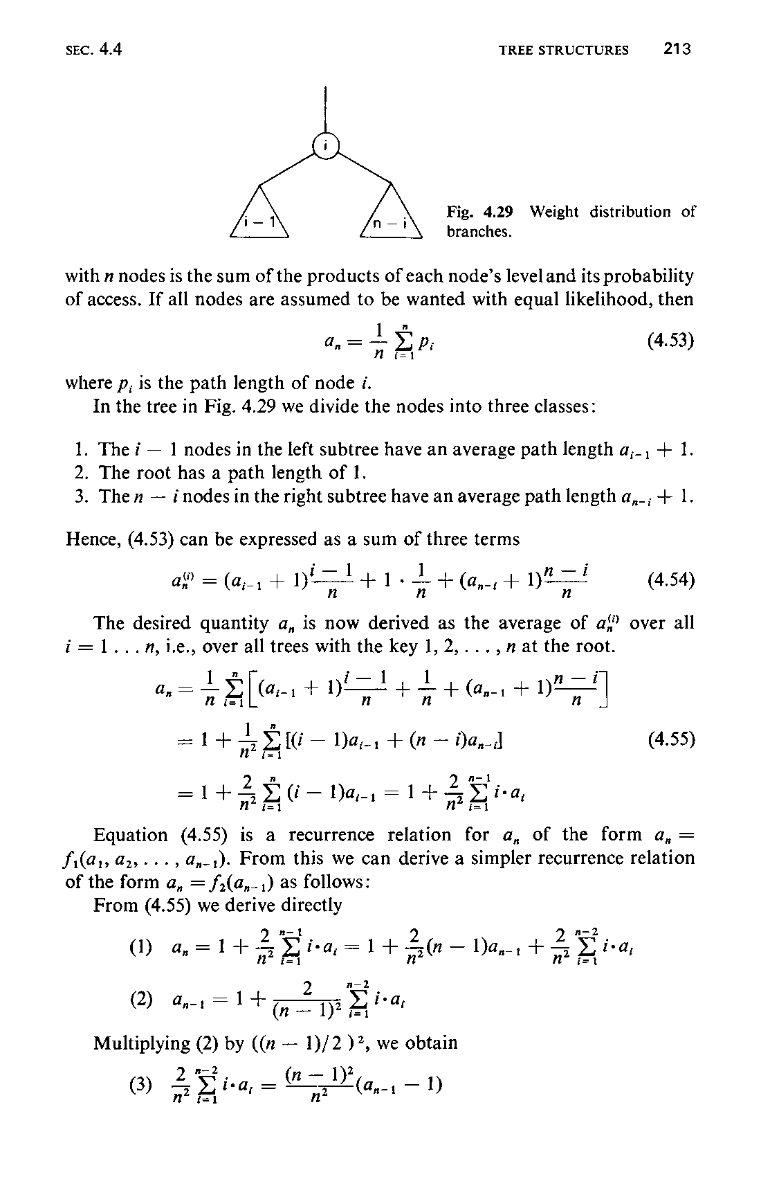
with n nodes is the sum of the products of each node’s level and its probability of access. If all nodes are assumed to be wanted with equal likelihood, then

1. The i — 1 nodes in the left subtree have an average path length a,_, + 1. 2. The root has a path length of 1.

2. Then — inodes in the right subtree have an average path length a,_; + 1.

The desired quantity a, is now derived as the average of a‘ over all i=1...n,1.e., over all trees with the a 1,2,..., at the root.

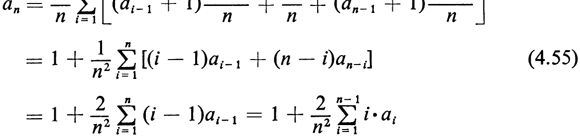
Equation (4.55) is a recurrence relation for a, of the form a, = Si(@1, @2,..., @,-1). From this we can derive a simpler recurrence relation of the form a, = f,(a,_,) as follows:

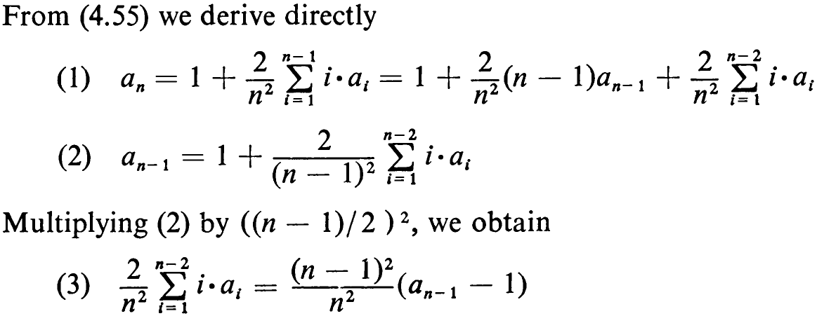
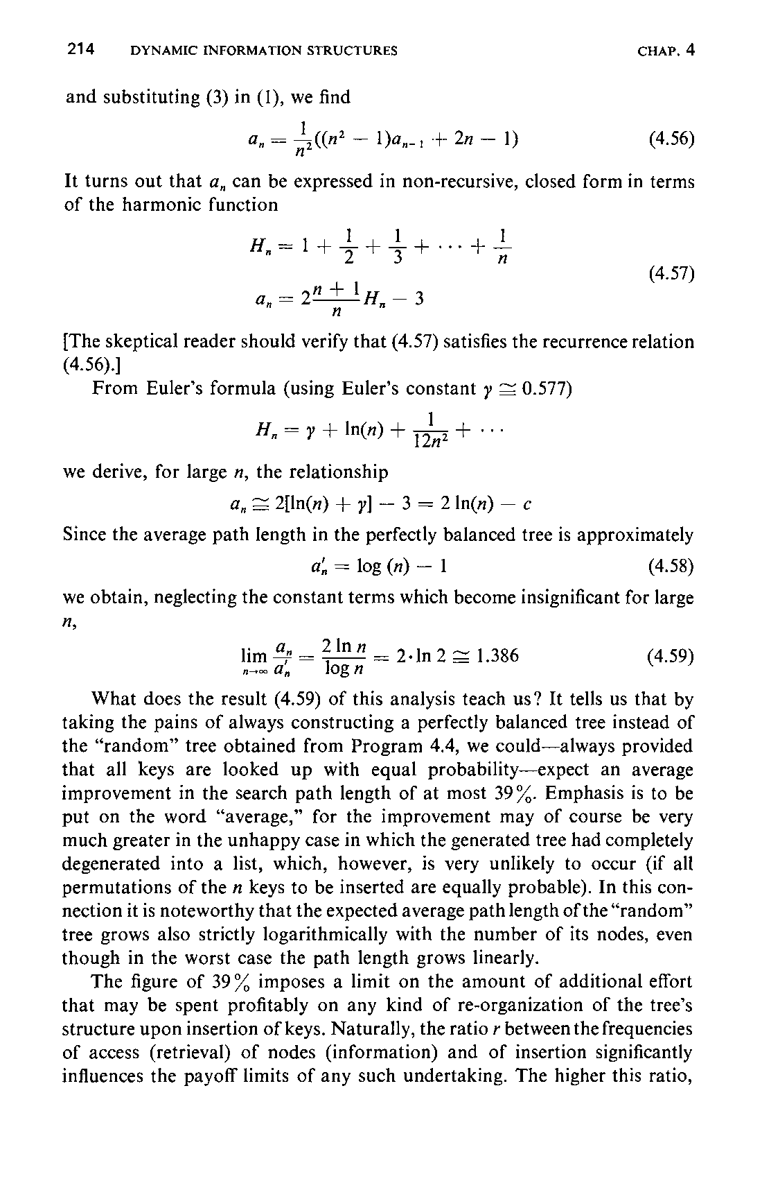
It turns out that a, can be expressed in non-recursive, closed form in terms of the harmonic function

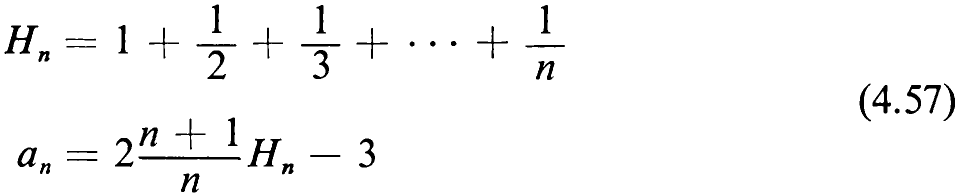
[The skeptical reader should verify that (4.57) satisfies the recurrence relation

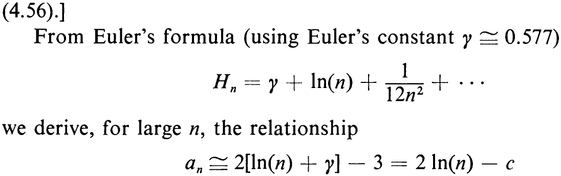
Since the average path length in the perfectly balanced tree is approximately

we obtain, neglecting the constant terms which become insignificant for large

What does the result (4.59) of this analysis teach us? It tells us that by taking the pains of always constructing a perfectly balanced tree instead of the “random” tree obtained from Program 4.4, we could—always provided that all keys are looked up with equal probability—expect an average improvement in the search path length of at most 39%. Emphasis is to be put on the word “average,” for the improvement may of course be very much greater in the unhappy case in which the generated tree had completely degenerated into a list, which, however, is very unlikely to occur (if all permutations of the n keys to be inserted are equally probable). In this connection it is noteworthy that the expected average path length of the “random” tree grows also strictly logarithmically with the number of its nodes, even though in the worst case the path length grows linearly.

The figure of 39% imposes a limit on the amount of additional effort that may be spent profitably on any kind of re-organization of the tree’s structure upon insertion of keys. Naturally, the ratio r between the frequencies of access (retrieval) of nodes (information) and of insertion significantly influences the payoff limits of any such undertaking. The higher this ratio,215 the higher is the payoff of a re-organization procedure. The 39% figure is low enough that in most applications improvements of the straight tree insertion algorithm do not pay off unless the number of nodes and the access vs. insertion ratio are large (or if one is afraid of the worst case).

4.4.6 Balanced Trees

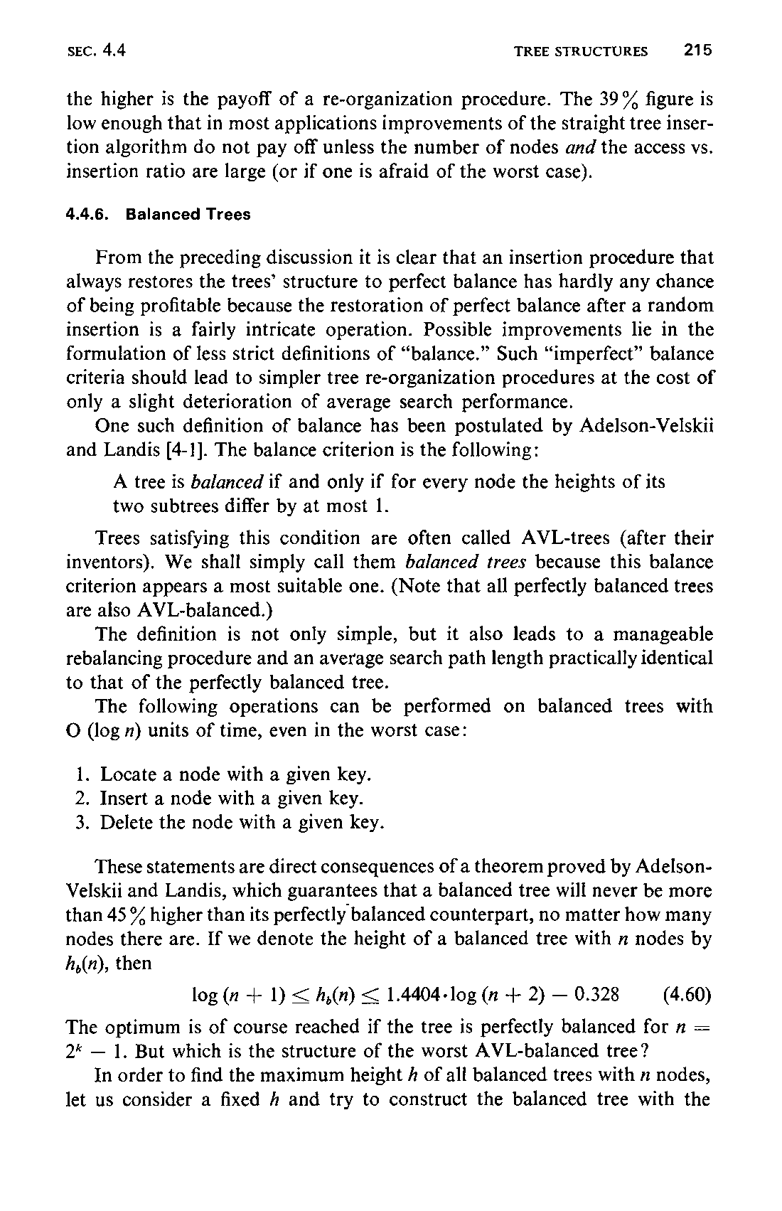
From the preceding discussion it is clear that an insertion procedure that always restores the trees’ structure to perfect balance has hardly any chance of being profitable because the restoration of perfect balance after a random insertion is a fairly intricate operation. Possible improvements lie in the formulation of less strict definitions of “balance.” Such “imperfect” balance criteria should lead to simpler tree re-organization procedures at the cost of only a slight deterioration of average search performance.

One such definition of balance has been postulated by Adelson-Velskii and Landis [4-1]. The balance criterion is the following:

Trees satisfying this condition are often called AVL-trees (after their inventors). We shall simply call them balanced trees because this balance criterion appears a most suitable one. (Note that all perfectly balanced trees are also AVL-balanced.)

The definition is not only simple, but it also leads to a manageable rebalancing procedure and an average search path length practically identical to that of the perfectly balanced tree.

The following operations can be performed on balanced trees with O (log 1) units of time, even in the worst case:

1. Locate a node with a given key.

2. Insert a node with a given key.

3. Delete the node with a given key.

These statements are direct consequences of a theorem proved by Adelson-Velskii and Landis, which guarantees that a balanced tree will never be more than 45 % higher than its perfectly balanced counterpart, no matter how many nodes there are. If we denote the height of a balanced tree with n nodes by h,(n), then

The optimum is of course reached if the tree is perfectly balanced for n = 2* — 1. But which is the structure of the worst AVL-balanced tree?

In order to find the maximum height A of all balanced trees with n nodes, let us consider a fixed A and try to construct the balanced tree with the216 minimum number of nodes. This strategy is recommended because, as in the case of the minimal A, the value can be attained only for certain specific values of n. Let this tree of height A be denoted by T;,. Clearly, T, is the empty tree, and 7, is the tree with a single node. In order to construct the tree 7, for h > 1, we will provide the root with two subtrees which again have a minimal number of nodes. Hence, the subtrees are also T’s. Evidently, one subtree must have height h — 1, and the other is then allowed to have a height of one less, i.e., of h — 2. Figure 4.30 shows the trees with height 2,

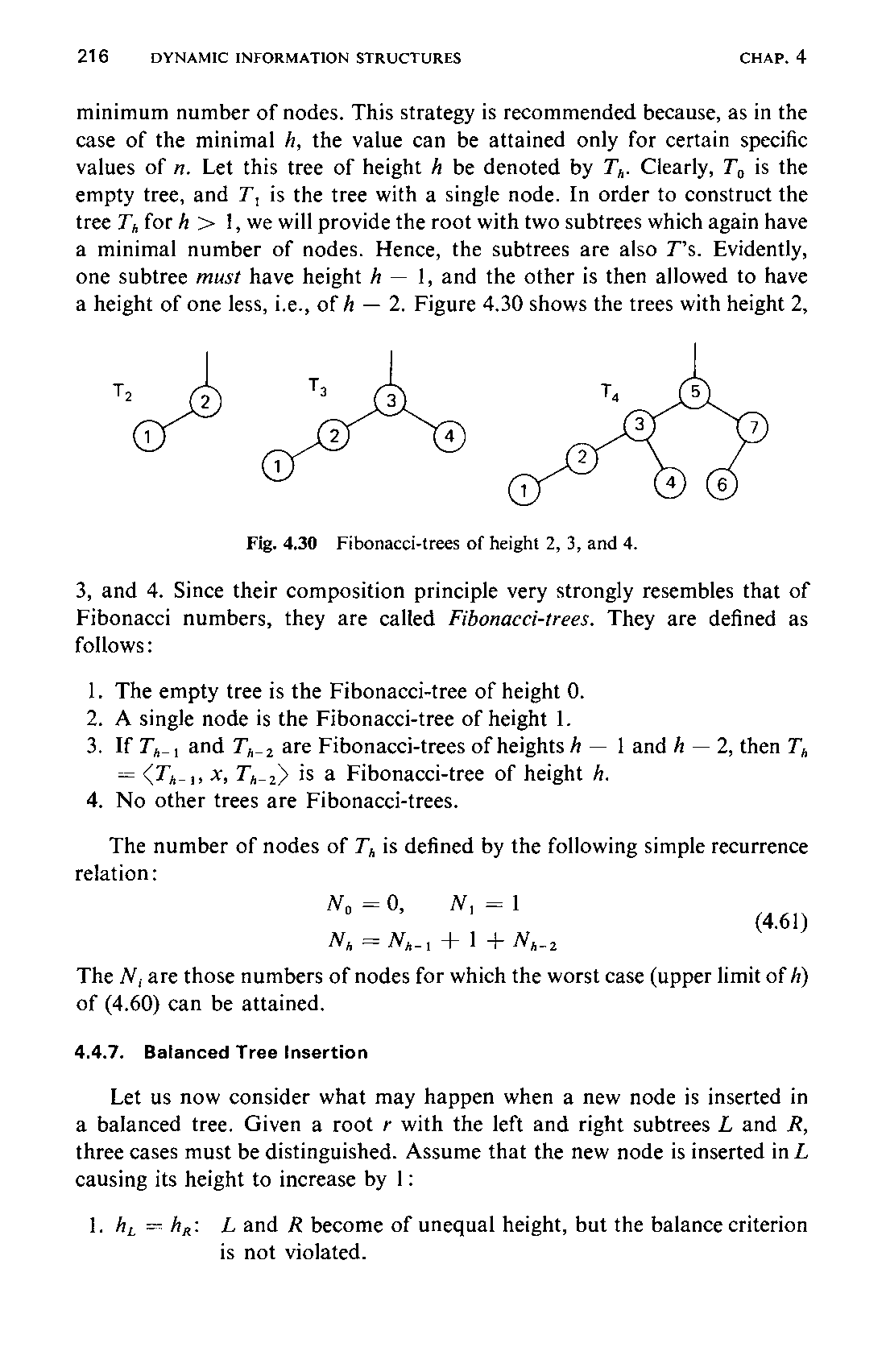
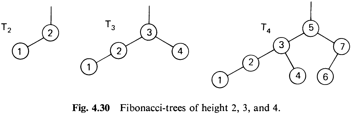
3, and 4. Since their composition principle very strongly resembles that of Fibonacci numbers, they are called Fibonacci-trees. They are defined as follows:

1. The empty tree is the Fibonacci-tree of height 0.

2. A single node is the Fibonacci-tree of height 1.

3. If T,., and 7,_, are Fibonacci-trees of heights h — 1 and A — 2, then T, = (T,_;, X, T,-2> is a Fibonacci-tree of height A.

4. No other trees are Fibonacci-trees.

The number of nodes of 7, is defined by the following simple recurrence relation:

The N; are those numbers of nodes for which the worst case (upper limit of /) of (4.60) can be attained.

4.4.7 Balanced Tree Insertion

Let us now consider what may happen when a new node is inserted in a balanced tree. Given a root r with the left and right subtrees L and R, three cases must be distinguished. Assume that the new node is inserted in L causing its height to increase by 1:

1. h, = hp: Land R become of unequal height, but the balance criterion is not violated.

2. hp <hg: Land R obtain equal height, i.e., the balance has even been improved.

3. hy, > hp: the balance criterion is violated, and the tree must be restructured.

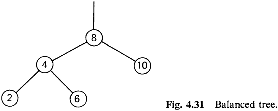
Consider the tree in Fig. 4.31. Nodes with keys 9 and 11 may be inserted without rebalancing; the tree with root 10 will become one-sided (case 1); the one with root 8 will improve its balance (case 2). Insertion of nodes 1, 3, 5, or 7, however, requires subsequent rebalancing.

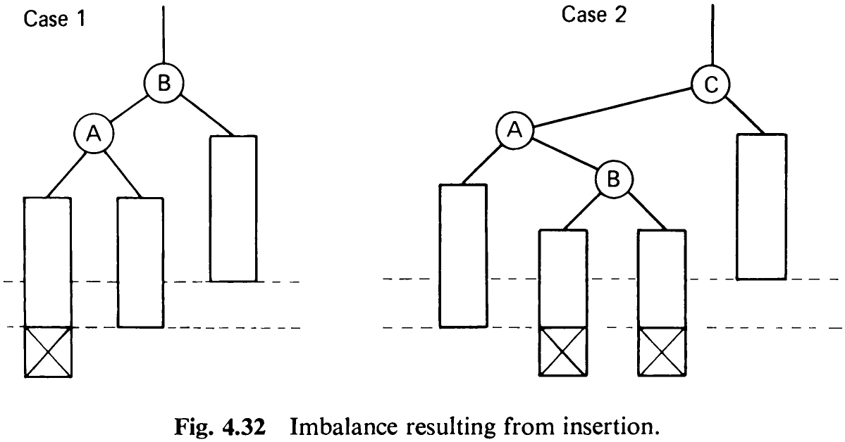
Some careful scrutiny of the situation reveals that there are only two essentially different constellations needing individual treatment. The remaining ones can be derived by symmetry considerations from those two. Case 1 is characterized by inserting keys 1 or 3 in the tree of Fig. 4.31, Case 2 by inserting nodes 5 or 7.

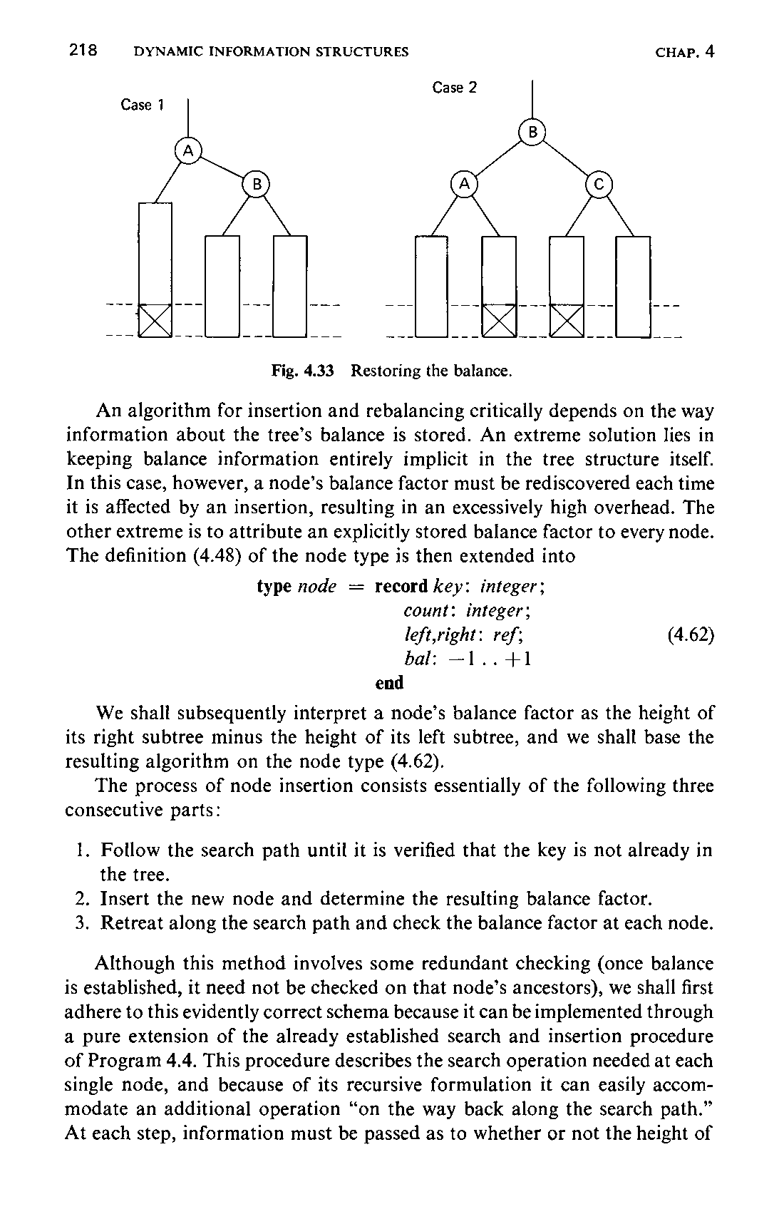
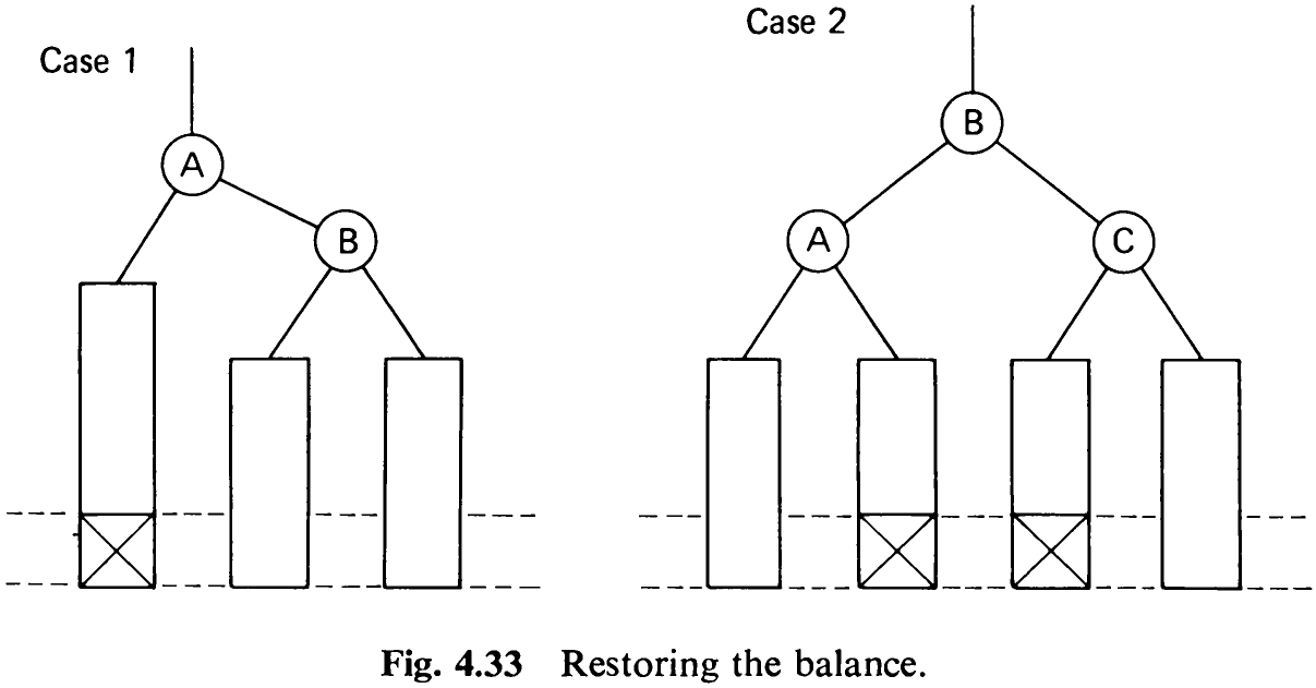
The two cases are generalized in Fig. 4.32 in which rectangular boxes denote subtrees, and the height added by the insertion is indicated by crosses. Simple transformations of the two structures restore the desired balance. Their result is shown in Fig. 4.33; note that the only movements allowed are those occurring in the vertical direction, whereas the relative horizontal positions of the shown nodes and subtrees must remain unchanged.

An algorithm for insertion and rebalancing critically depends on the way information about the tree’s balance is stored. An extreme solution lies in keeping balance information entirely implicit in the tree structure itself. In this case, however, a node’s balance factor must be rediscovered each time it is affected by an insertion, resulting in an excessively high overhead. The other extreme is to attribute an explicitly stored balance factor to every node. The definition (4.48) of the node type is then extended into

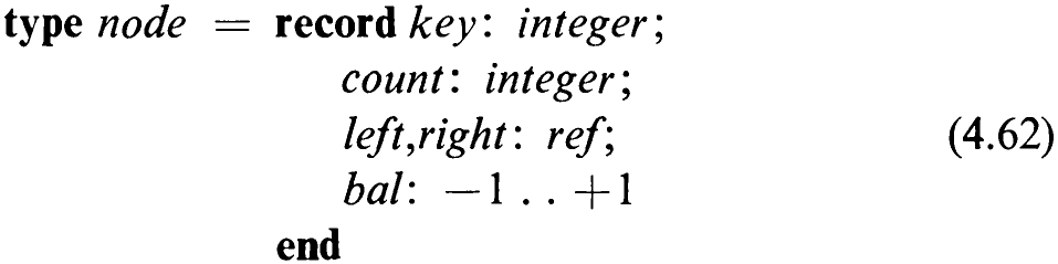
We shall subsequently interpret a node’s balance factor as the height of its right subtree minus the height of its left subtree, and we shall base the resulting algorithm on the node type (4.62).

The process of node insertion consists essentially of the following three consecutive parts:

1. Follow the search path until it is verified that the key is not already in the tree.

2. Insert the new node and determine the resulting balance factor.

3. Retreat along the search path and check the balance factor at each node.

Although this method involves some redundant checking (once balance is established, it need not be checked on that node’s ancestors), we shall first adhere to this evidently correct schema because it can be implemented through a pure extension of the already established search and insertion procedure of Program 4.4. This procedure describes the search operation needed at each single node, and because of its recursive formulation it can easily accommodate an additional operation “on the way back along the search path.” At each step, information must be passed as to whether or not the height of219 the subtree (in which the insertion had been performed) had increased. We therefore extend the procedure’s parameter list by the Boolean A with the meaning “the subtree height has increased.” Clearly, h must denote a variable parameter since it is used to transmit a result.

Assume now that the process is returning to a node pt from the left branch (see Fig. 4.32), with the indication that it has increased its height. We now must distinguish between the three situations involving the subtree heights prior to insertion:

l. hy < hg, p}.bal = +1, the previous imbalance at p has been equilibrated. 2. hy = ha, pt.bal = 0, the weight is now slanted to the left.

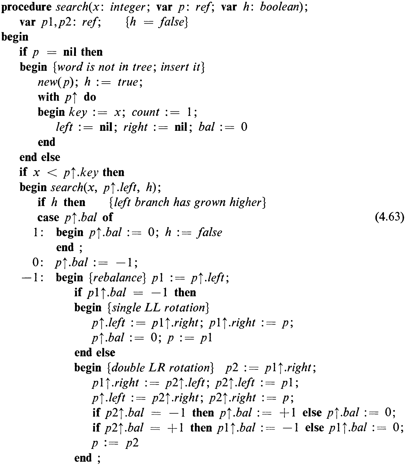
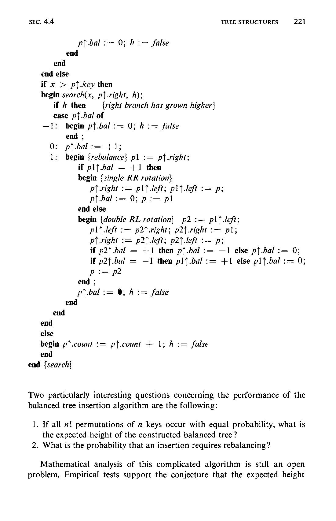
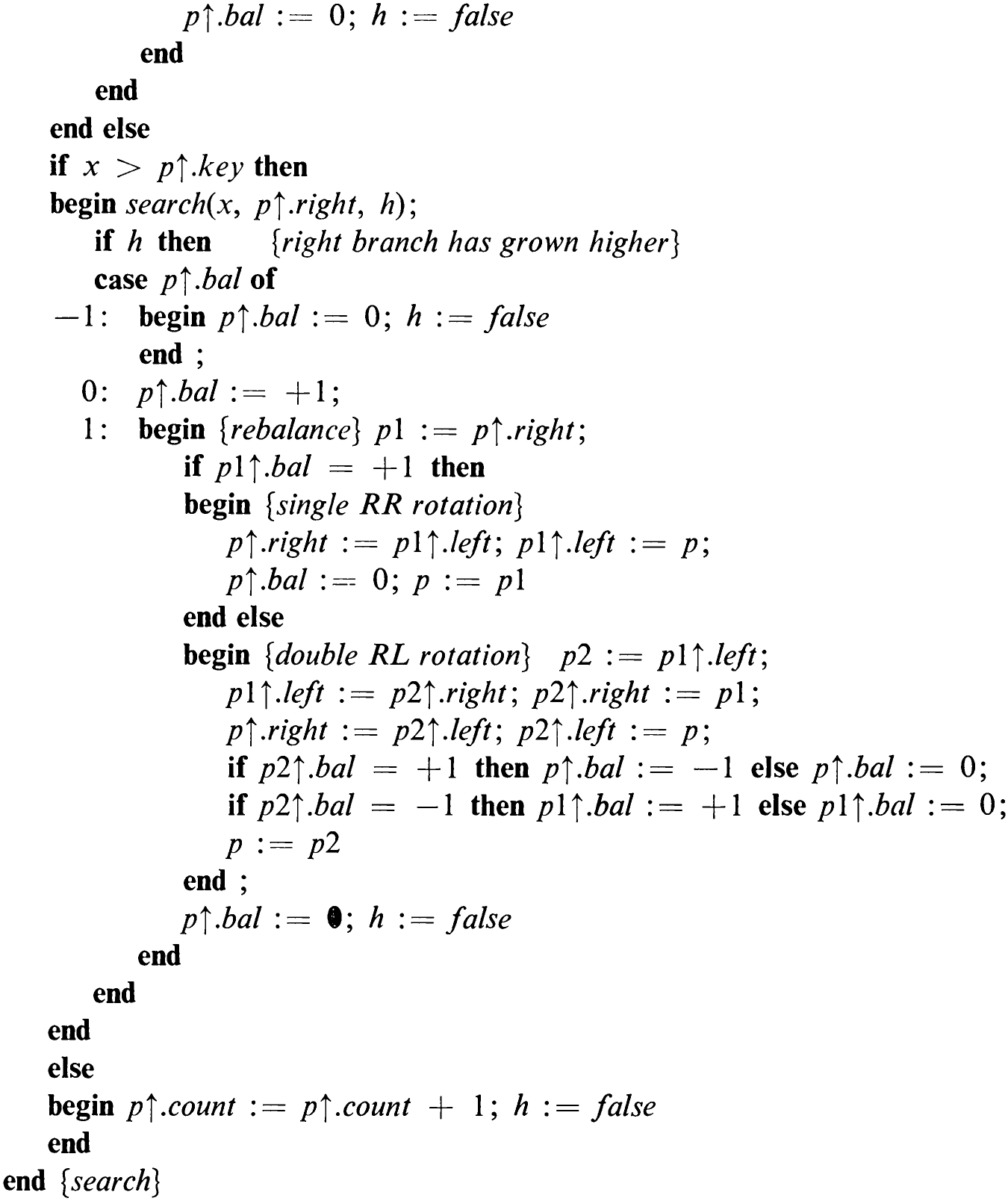
In the third case, inspection of the balance factor of the root of the left subtree (say, plt.bal) determines whether case 1 or case 2 of Fig. 4.32 is present. If that node has also a higher left than right subtree, then we have to deal with case 1, otherwise with case 2. (Convince yourself that a left subtree with a balance factor equal to 0 at its root cannot occur in this case.) The rebalancing operations necessary are entirely expressed as sequences of pointer re-assignments. In fact, pointers are cyclically exchanged, resulting in either a single or a double rotation of the two or three nodes involved. In addition to pointer rotation, the respective node balance factors also have to be adjusted. The details are shown in the search, insertion, and rebalancing procedure (4.63).

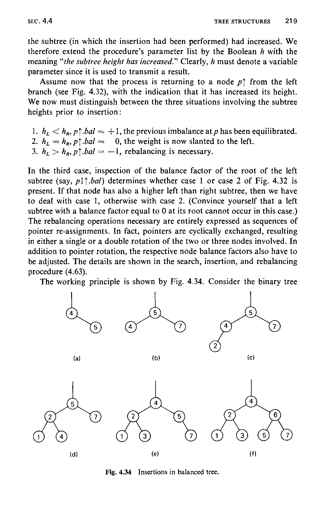
The working principle is shown by Fig. 4.34. Consider the binary tree

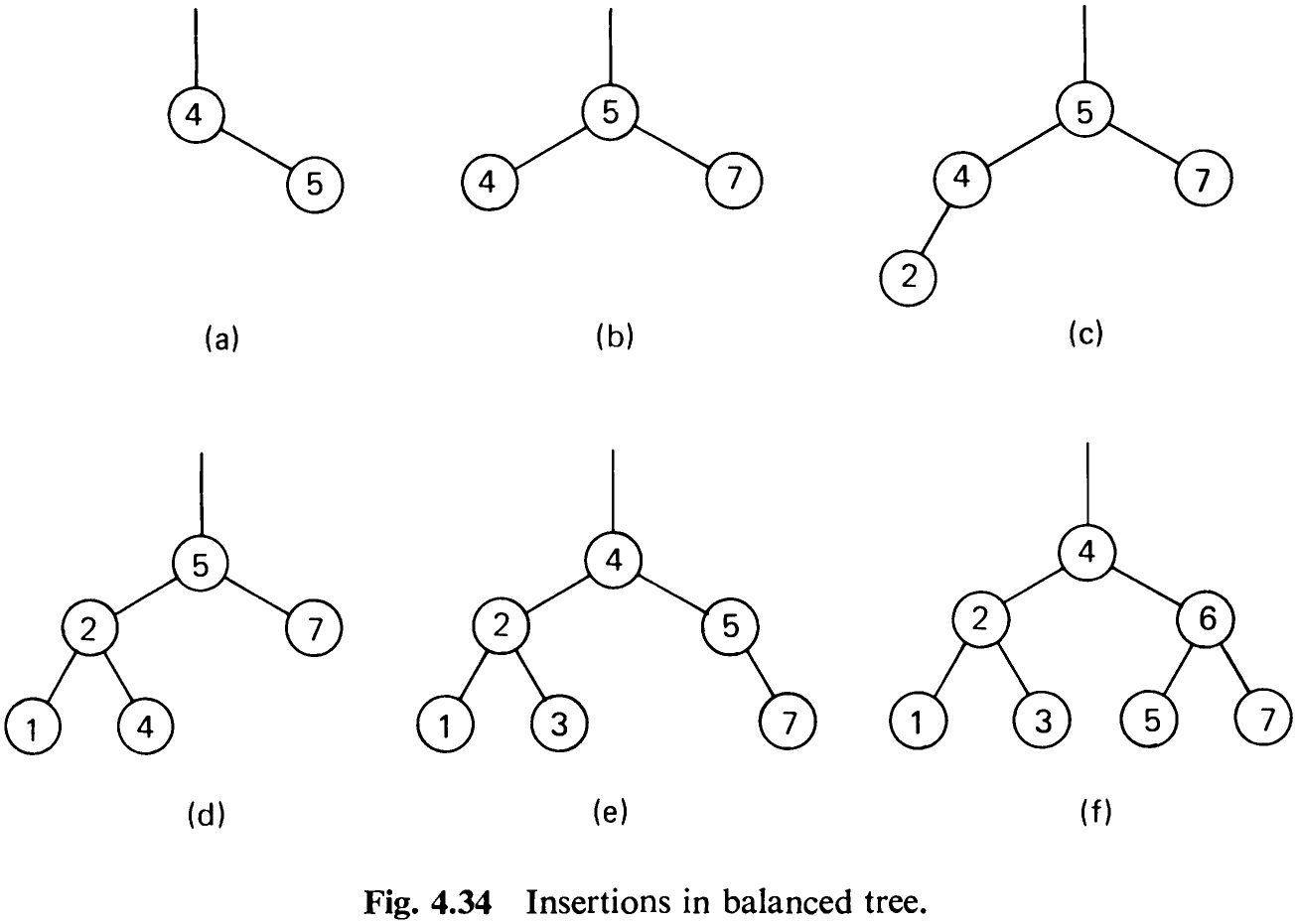
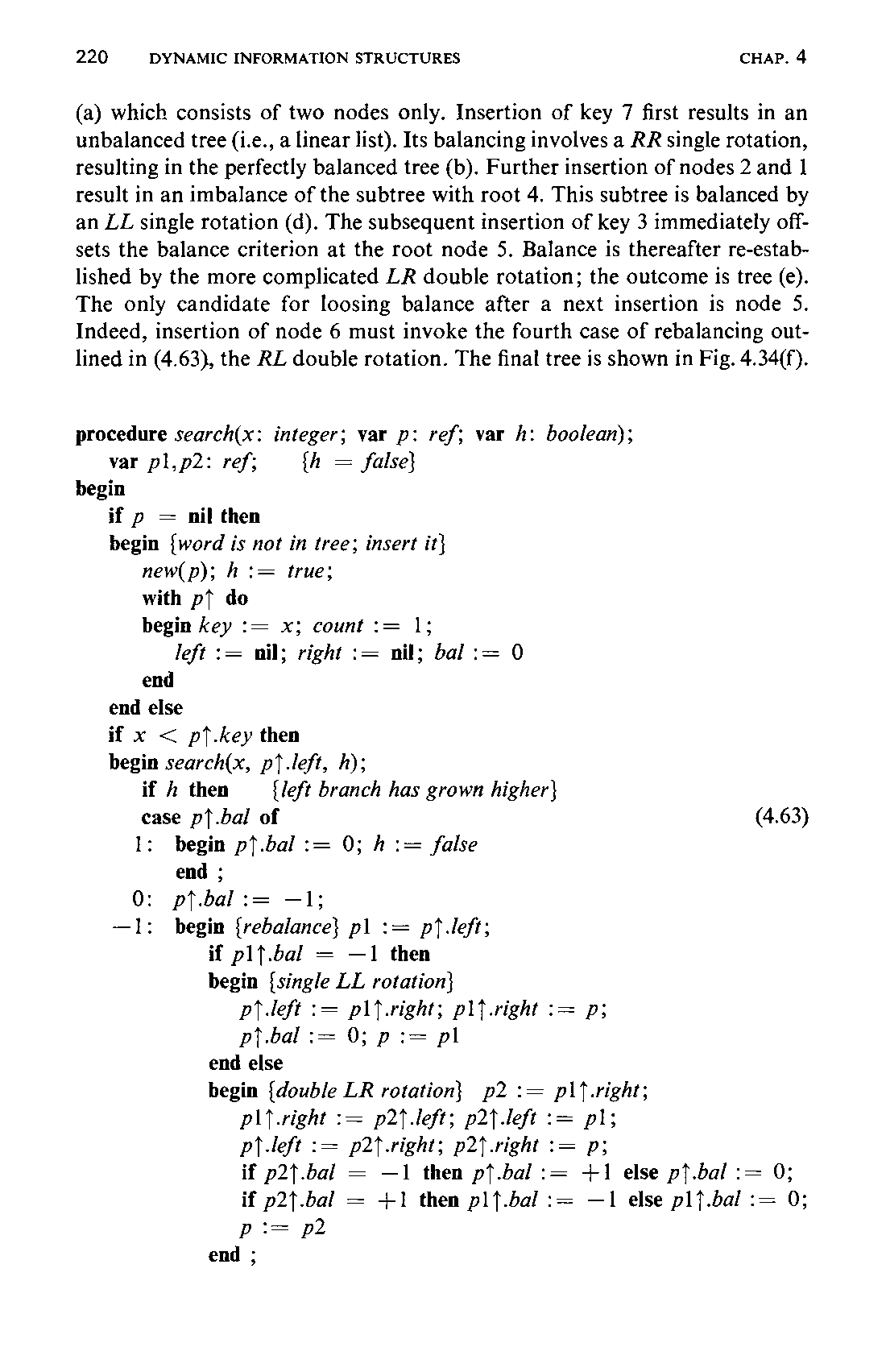
(a) which consists of two nodes only. Insertion of key 7 first results in an unbalanced tree (i.e., a linear list). Its balancing involves a RR single rotation, resulting in the perfectly balanced tree (b). Further insertion of nodes 2 and 1 result in an imbalance of the subtree with root 4. This subtree is balanced by an LL single rotation (d). The subsequent insertion of key 3 immediately offsets the balance criterion at the root node 5. Balance is thereafter re-established by the more complicated LR double rotation; the outcome is tree (e). The only candidate for loosing balance after a next insertion is node 5. Indeed, insertion of node 6 must invoke the fourth case of rebalancing outlined in (4.63), the RL double rotation. The final tree is shown in Fig. 4.34(f).

Two particularly interesting questions concerning the performance of the balanced tree insertion algorithm are the following:

1. If all ! permutations of n keys occur with equal probability, what is the expected height of the constructed balanced tree?

2. What is the probability that an insertion requires rebalancing ?

Mathematical analysis of this complicated algorithm is still an open problem. Empirical tests support the conjecture that the expected height222 of the balanced tree generated by (4.63) is A = log (m) + c, where c isa small constant (c = 0.25). This means that in practice the AVL-balanced tree behaves as well as the perfectly balanced tree, although it is much simpler to maintain. Empirical evidence also suggests that, on the average, rebalancing is necessary once for approximately every two insertions. Here single and double rotations are equally probable. The example of Fig. 4.34 has evidently been carefully chosen to demonstrate as many rotations as possible in a minimum number of insertions!

The complexity of the balancing operations suggests that balanced trees should be used only if information retrievals are considerably more frequent than insertions. This is particularly true because the nodes of such search trees are usually implemented as densely packed records in order to economize storage. The speed of access and of updating the balance factors—each requiring two bits only—is therefore often a decisive factor to the efficiency of the rebalancing operation. Empirical evaluations show that balanced trees lose much of their appeal if tight record packing is mandatory. It is indeed difficult to beat the straightforward, simple tree insertion algorithm!

4.4.8 Balanced Tree Deletion

Our experience with tree deletion suggests that in the case of balanced trees deletion will also be more complicated than insertion. This is indeed true, although the rebalancing operation remains essentially the same as for insertion. In particular, rebalancing consists of either a single or a double rotation of nodes.

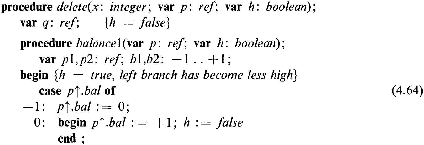
The basis for balanced tree deletion is algorithm (4.52). The easy cases are terminal nodes and nodes with only a single descendant. If the node to be deleted has two subtrees, we will again replace it by the rightmost node of its left subtree. As in the case of insertion (4.63), a Boolean variable parameter / is added with the meaning “the height of the subtree has been reduced.” Rebalancing has to be considered only when / is true. A is assigned the value true upon finding and deleting a node or if rebalancing itself reduces the height of a subtree. In (4.64) we introduce the two (symmetric) balancing operations in the form of procedures since they have to be invoked from more than one place in the deletion algorithm. Note that balance/ is applied when the left, balance2 after the right branch had been reduced in height.

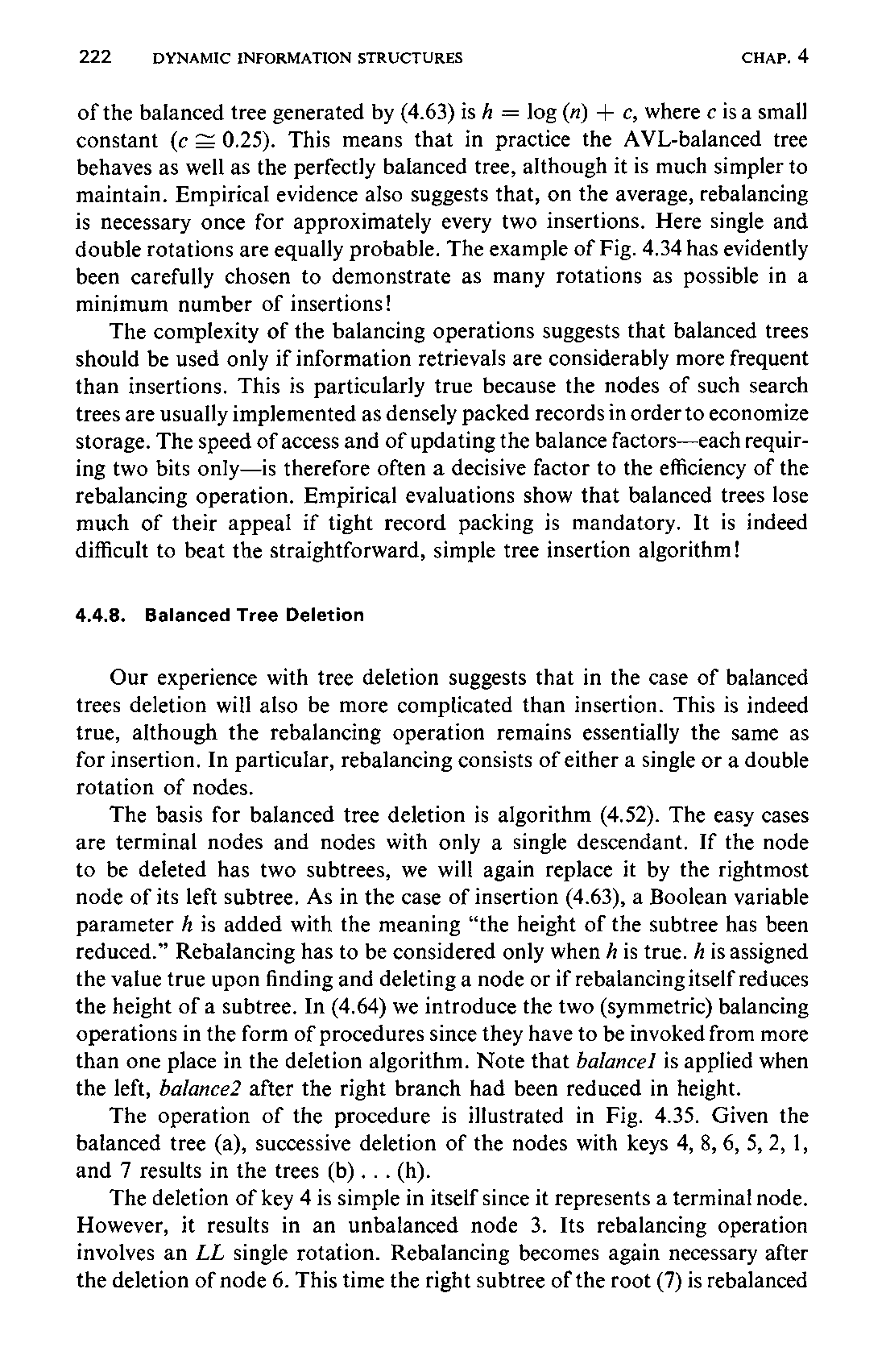
The operation of the procedure is illustrated in Fig. 4.35. Given the balanced tree (a), successive deletion of the nodes with keys 4, 8, 6, 5, 2, 1, and 7 results in the trees (b)... (h).

The deletion of key 4 is simple in itself since it represents a terminal node. However, it results in an unbalanced node 3. Its rebalancing operation involves an LL single rotation. Rebalancing becomes again necessary after the deletion of node 6. This time the right subtree of the root (7) is rebalanced

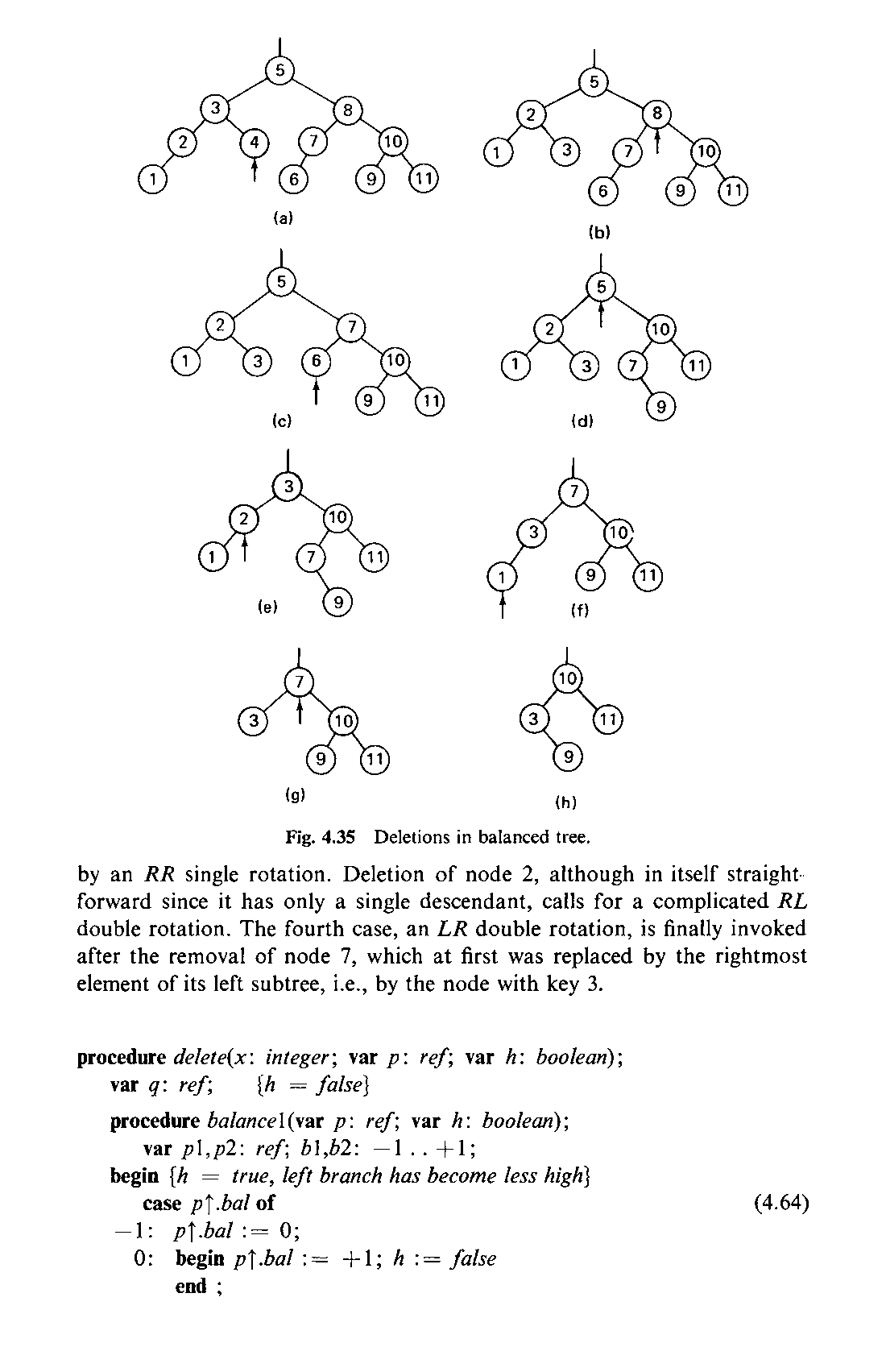
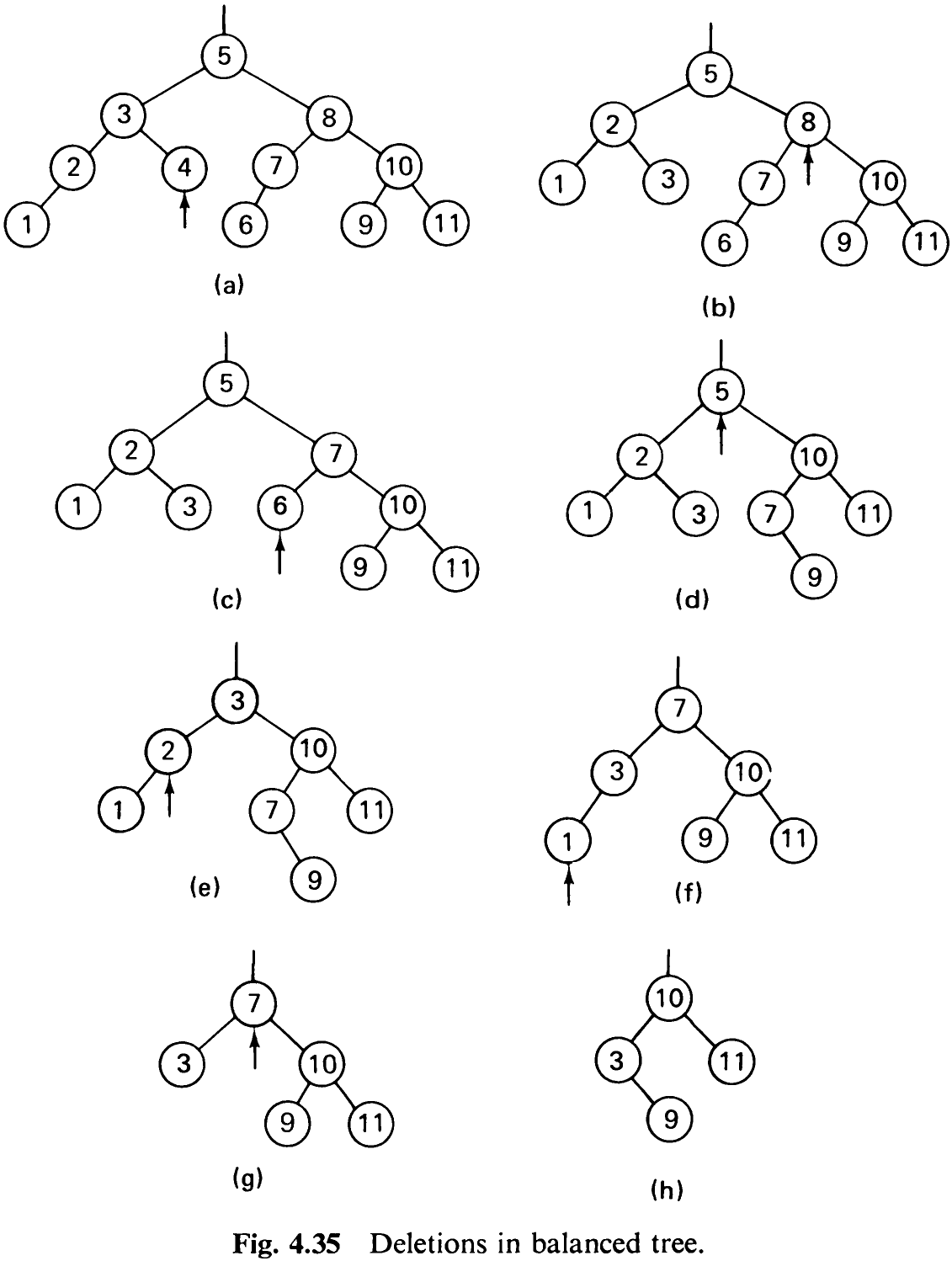
by an RR single rotation. Deletion of node 2, although in itself straightforward since it has only a single descendant, calls for a complicated RL double rotation. The fourth case, an LR double rotation, is finally invoked after the removal of node 7, which at first was replaced by the rightmost element of its left subtree, i.e., by the node with key 3.

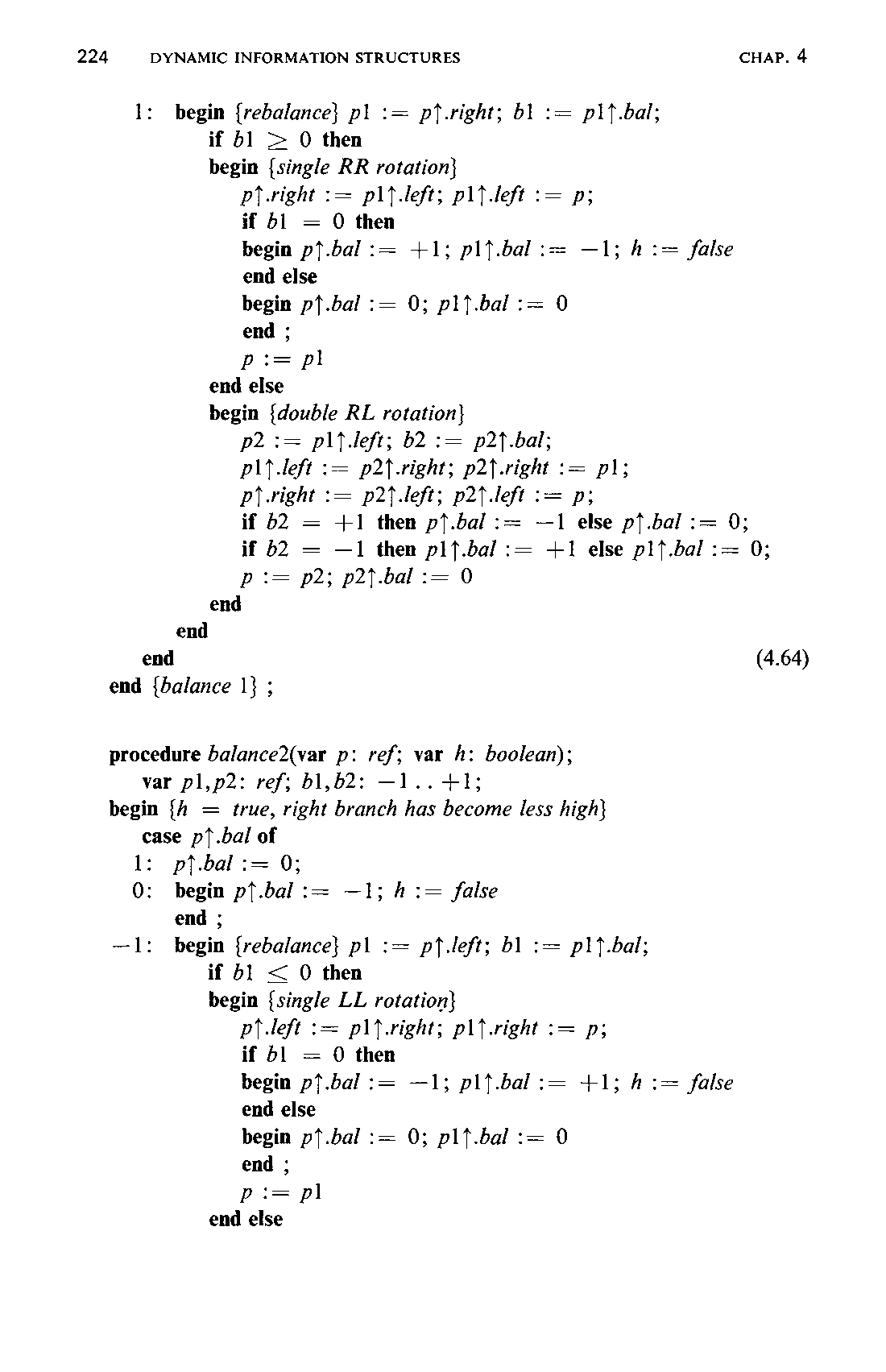
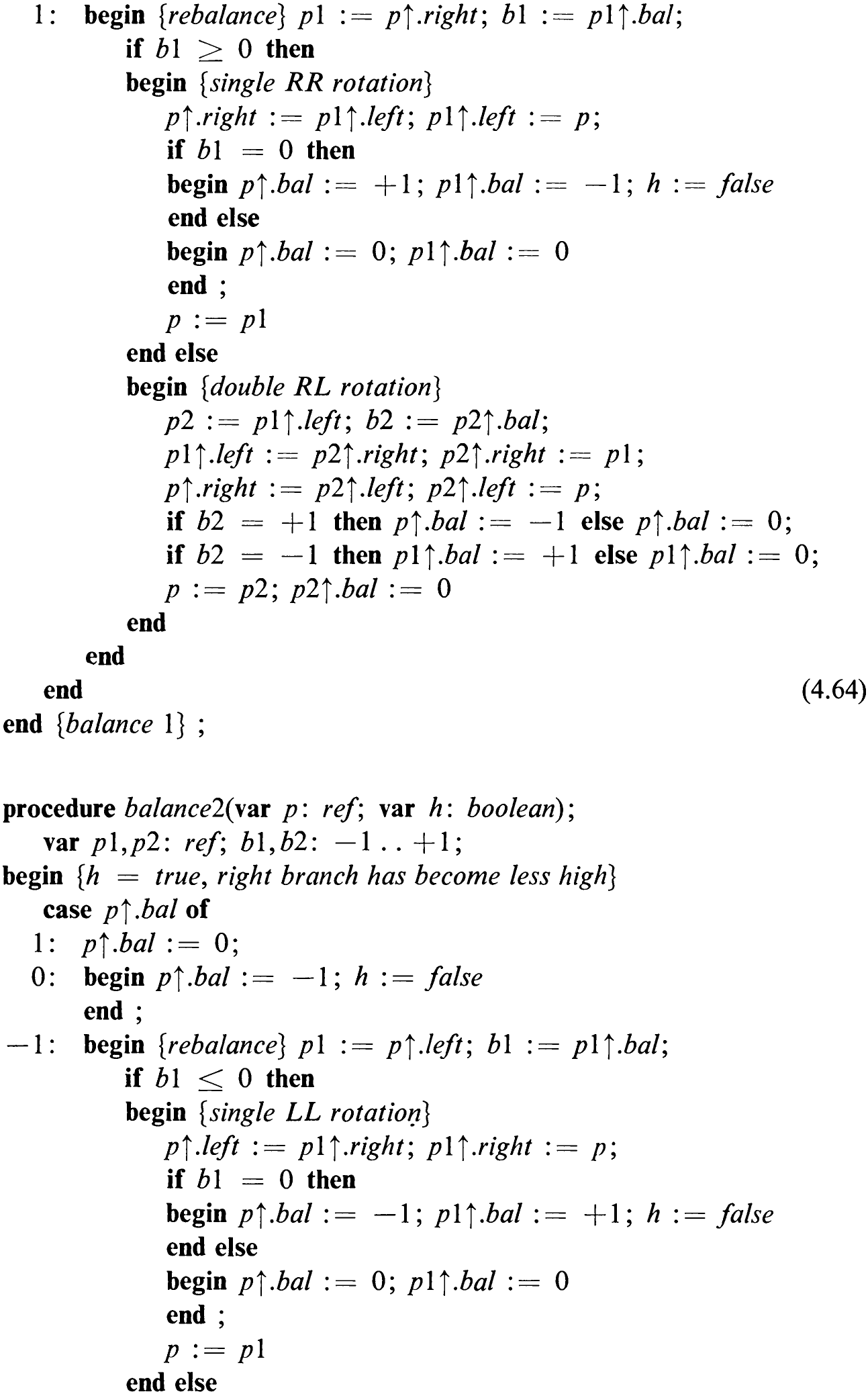
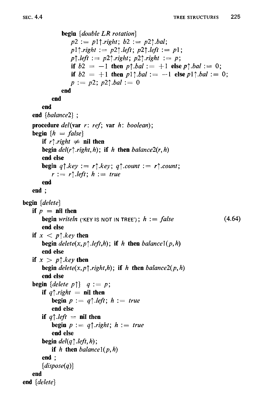
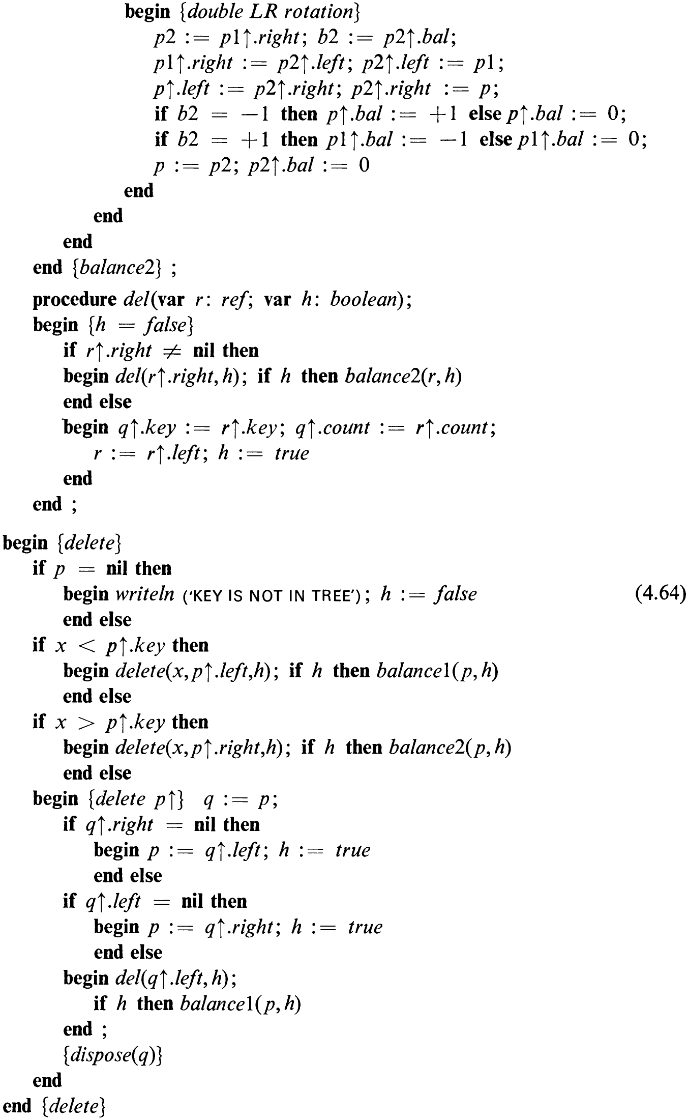
Evidently, deletion of an element in a balanced tree can also be performed with—in the worst case—O (log) operations. An essential difference between the behavior of the insertion and deletion procedures must not be overlooked, however. Whereas insertion of a single key may result in at most one rotation (of two or three nodes), deletion may require a rotation at every node along the search path. Consider, for instance, deletion of the rightmost node of a Fibonacci-tree. In this case the deletion of any single node leads to a reduction of the height of the tree; in addition, deletion of its rightmost node requires the maximum number of rotations. This therefore represents the worst choice of node in the worst case of a balanced tree, a rather unlucky combination of chances! How probable are rotations, then, in general? The surprising result of empirical tests is that whereas one rotation is invoked for approximately every two insertions, one is required for every five deletions only. Deletion in balanced trees is therefore about as easy—or as complicated —as insertion.

4.4.9 Optimal Search Trees

So far our consideration of organizing search trees has been based on the assumption that the frequency of access is equal for all nodes, that is, that all keys are equally probable to occur as a search argument. This is probably the best assumption if one has no idea of access distribution. However, there are cases (they are the exception rather than the rule) in which information on the probabilities of access to individual keys is available. These cases usually have the characteristic that the keys always remain the same, i.e., the search tree is subjected neither to insertions nor to deletions, but retains a constant structure. A typical example is the scanner of a compiler which determines for each word (identifier) whether or not it is a keyword (reserved word). Statistical measurements over hundreds of compiled programs may in this case yield accurate information on the relative frequencies of occurrence, and thereby of access, of individual keys.

Assume that in a search tree the probability with which node i is accessed iS D,.

We now wish to organize the search tree in a way that the total number of search steps—counted over sufficiently many trials—becomes minimal. For this purpose the definition of path length (4.34) is modified by attributing a certain weight to each node. Nodes which are frequently accessed become heavy nodes; those which are rarely visited become light nodes. The (internal) weighted path length is then the sum of all paths from the root to each node weighted by that node’s probability of access.

h, is the level of node i (or its distance from the root +1). The goal is now to minimize the weighted path length for a given probability distribution.

As an example, consider the set of keys 1, 2, 3, with probabilities of access DP, = 1/7, p, = 2/7, and p; = 4/7. These three keys can be arranged in five different ways as search trees (see Fig. 4.36).

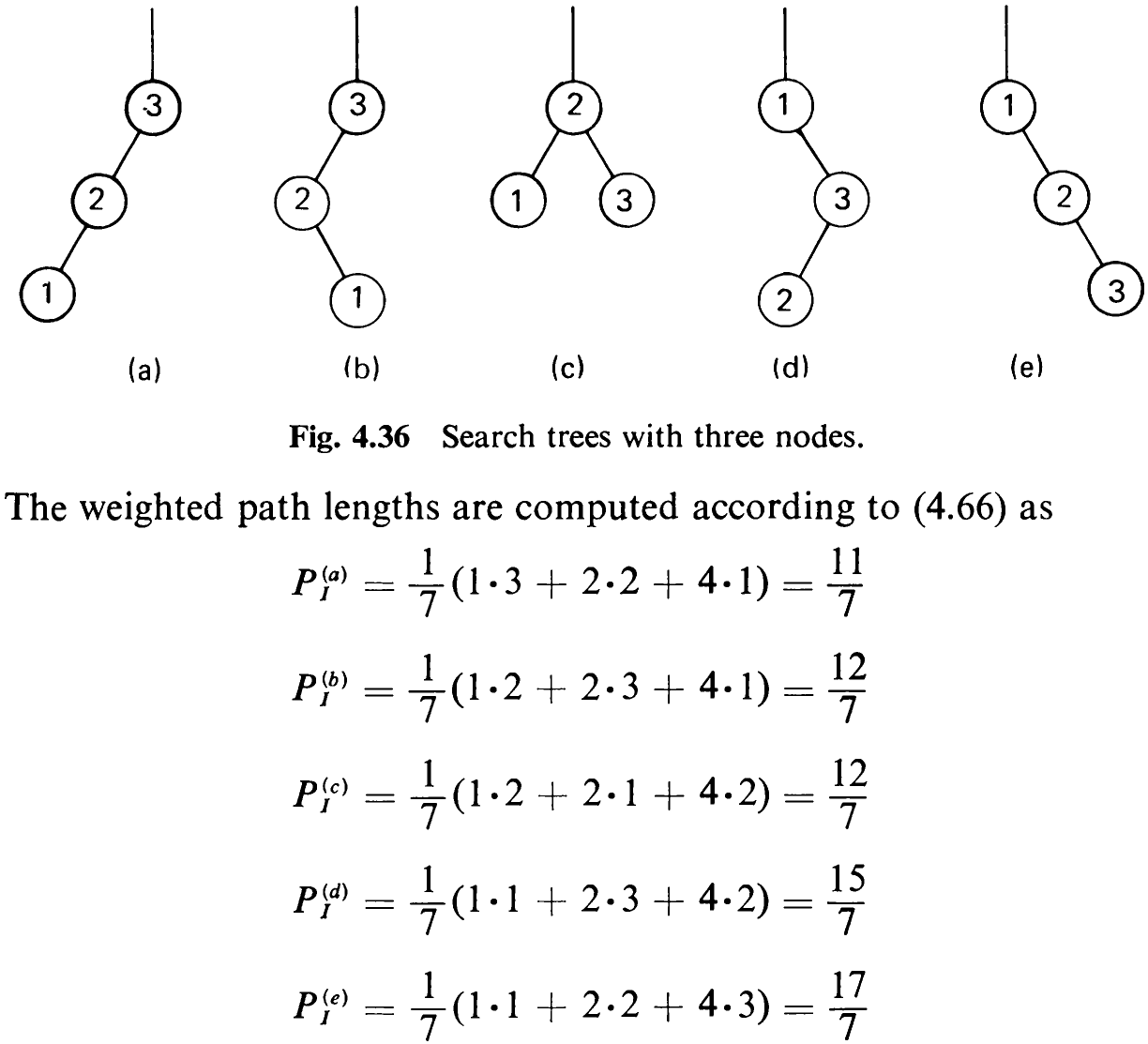
Hence, in this example not the perfectly balanced but the degenerate tree (a) turns out to be the optimal arrangement.

The example of the compiler scanner immediately suggests that this problem should be viewed under a slightly more general condition: Words occurring in the source text are not always keywords; as a matter of fact, their being keywords is rather the exception. Finding that a given word k is not a key in the search tree can be considered as an access to a hypothetical “special node” inserted between the next lower and next higher key (see Fig. 4.19) with an associated external path length. If the probability q, of a search argument x lying between the two keys k; and k;,, is also known, this information may considerably change the structure of the optimal search tree. Hence, we generalize the problem by also considering unsuccessful searches.

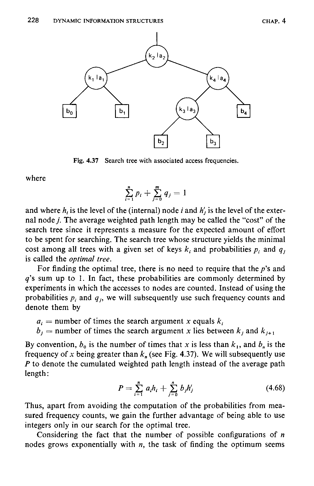
and where h, is the level of the (internal) node i and his the level of the external node j. The average weighted path length may be called the “cost” of the search tree since it represents a measure for the expected amount of effort to be spent for searching. The search tree whose structure yields the minimal cost among all trees with a given set of keys k, and probabilities p, and q, is called the optimal tree.

For finding the optimal tree, there is no need to require that the p’s and q’s sum up to 1. In fact, these probabilities are commonly determined by experiments in which the accesses to nodes are counted. Instead of using the probabilities p, and g,, we will subsequently use such frequency counts and denote them by

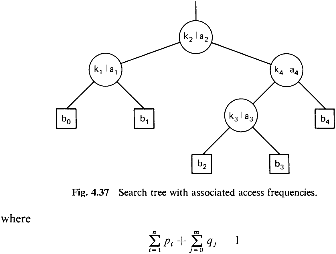
By convention, b, is the number of times that x is less than k,, and 8, is the frequency of x being greater than k, (see Fig. 4.37). We will subsequently use P to denote the cumulated weighted path length instead of the average path length:

Thus, apart from avoiding the computation of the probabilities from measured frequency counts, we gain the further advantage of being able to use integers only in our search for the optimal tree.

Considering the fact that the number of possible configurations of n nodes grows exponentially with n, the task of finding the optimum seems229 rather hopeless for large n. Optimal trees, however, have one significant property that helps to find them: all their subtrees are optimal too. For instance, if the tree in Fig. 4.37 is optimal for given a’s and b’s, then the subtree with keys k; and k, is also optimal as shown. This property suggests an algorithm that systematically finds larger and larger trees, starting with individual nodes as smallest possible subtrees. The tree thus grows “from the leaves to the root,” which is, since we are used to drawing trees upside-down, the “bottom-up” direction [4-6].

The equation that is the key to this algorithm is (4.69). Let P be the weighted path length of a tree, and let P, and P, be those of the left and right subtrees of its root. Clearly, P is the sum of P, and P, and the number of times a search travels on the single leg to the root, which is simply the total number W of search trials.

We call W the weight of the tree. Its average path length is then P/W.

These considerations show the need for a denotation of the weights and the path lengths of any subtree consisting of a number of adjacent keys. Let w;, denote the weight and let p,, denote the path length of the optimal subtree 7;, consisting of nodes with keys k;41, K;+2,...,k;. These quantities are defined by the recurrence relations (4.71) and (4.72)

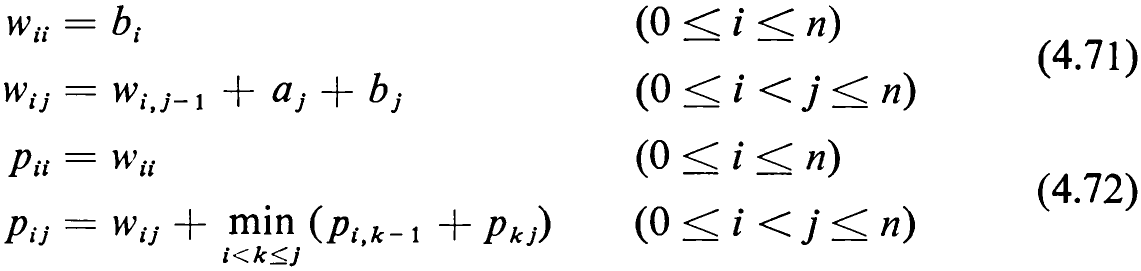
The last equation follows immediately from (4.69) and the definition of optimality.

Since there are approximately (1/2)n? values p,,, and since (4.72) calls for a choice among 0 <j —i<n cases, the minimization operation will involve approximately (1/6)? operations. Knuth pointed out that a factor n can be saved by the following consideration, which alone saves this algorithm for practical purposes.

Let r,, be a value of k which achieves the minimum in (4.72). It is possible to limit the search for r,, to a much smaller interval, i.e., to reduce the number of the j — i evaluation steps. The key is the observation that if we have found the root r,;; of the optimal subtree T,,, then neither extending the tree by adding a node to the right nor removing its leftmost node ever can cause the root to move to the left. This is expressed by the relation

which limits the search for possible solutions for r;; to the range r;j;-;... r;+1,;, and it results in a total number of elementary steps to O(n”). We are now ready to construct the optimization algorithm in detail. We recall the following definitions which are based on optimal trees 7,, consisting of nodes with keys k;,,...k;.

1. a,;: the frequency of a search for k;.

2. b,: the frequency of a search argument x between k, and k,,,.

3. w,,;: the weight of T,,.

4. p,;: the weighted path length of 7;,.

5. r,;: the index of the root of T;,.

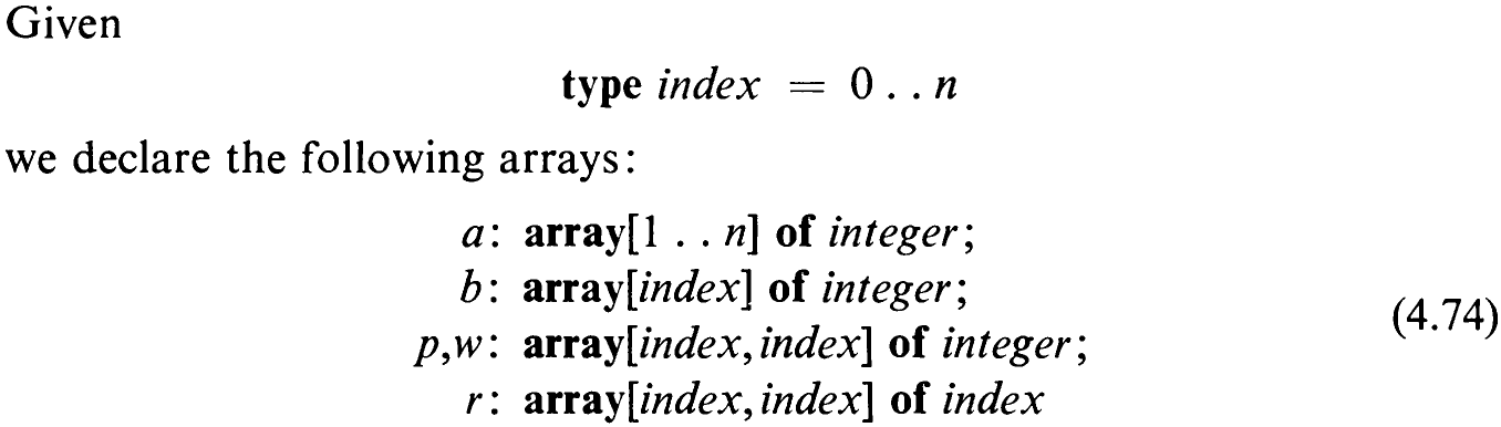
Assume that the weight w;,; has been computed from a and b in a straightforward way [see (4.71)]. Now consider w as the argument of the procedure to be developed and consider r as its result, for r describes the structure completely. p may be considered an intermediate result. Starting out by considering the smallest possible subtrees, namely, those consisting of no nodes at all, we proceed to larger and larger trees. Let us denote the width j — i of the subtree 7;, by A. Then we can trivially determine the values p,; for all trees with A = 0 according to (4.72).

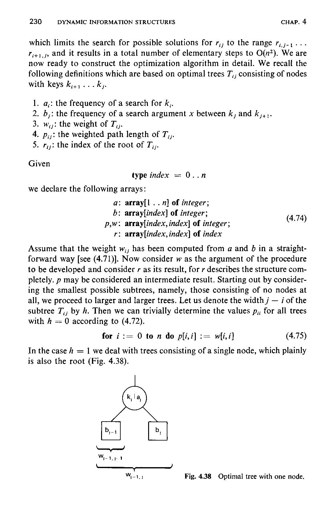
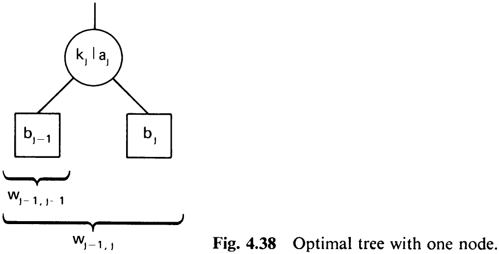
In the case h = 1 we deal with trees consisting of a single node, which plainly is also the root (Fig. 4.38).

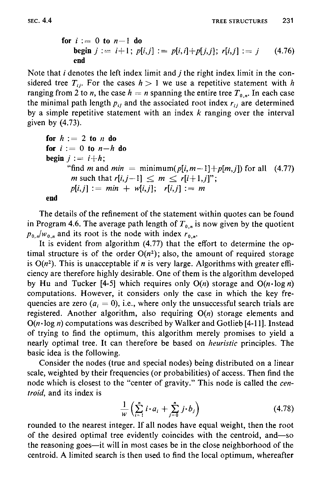
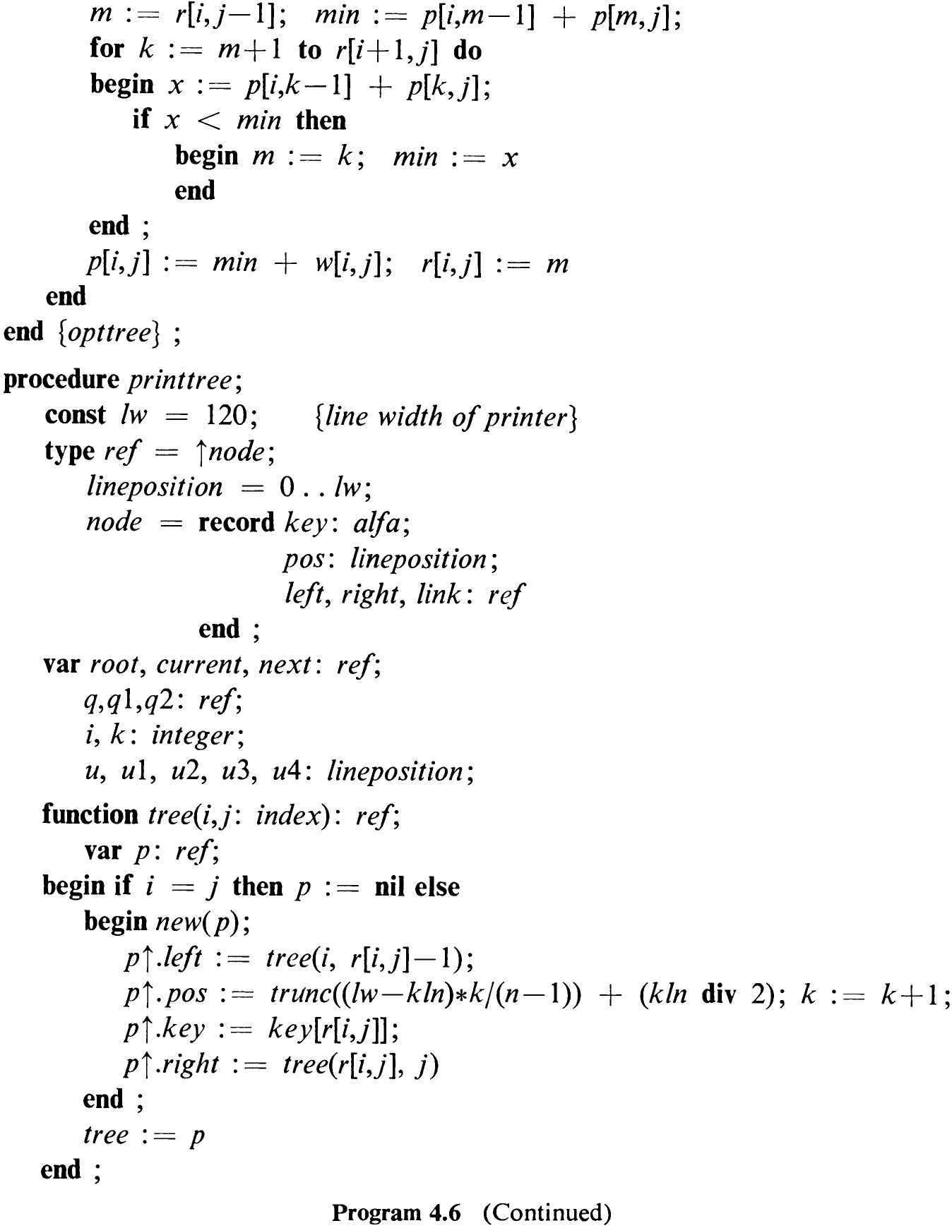
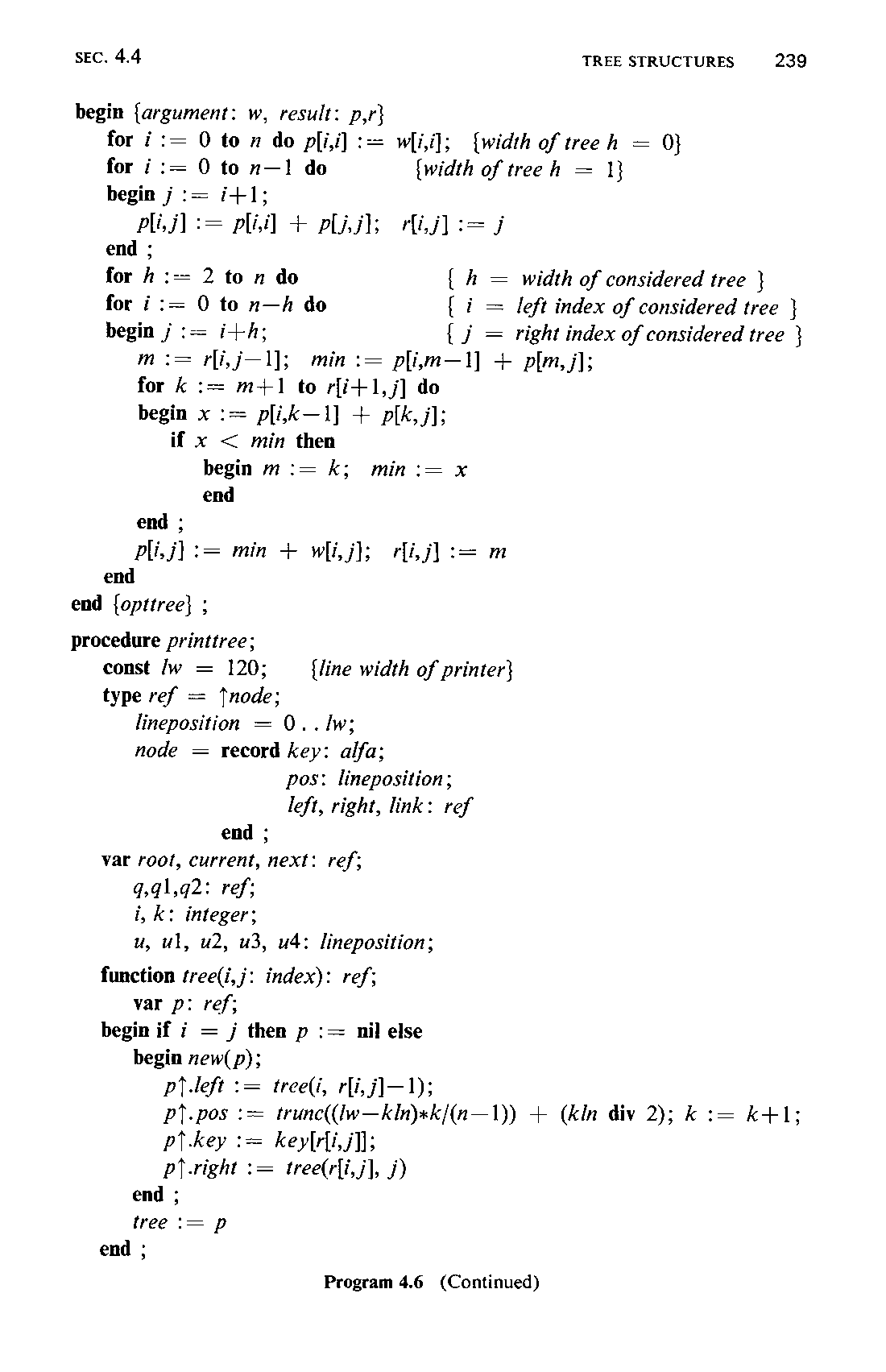
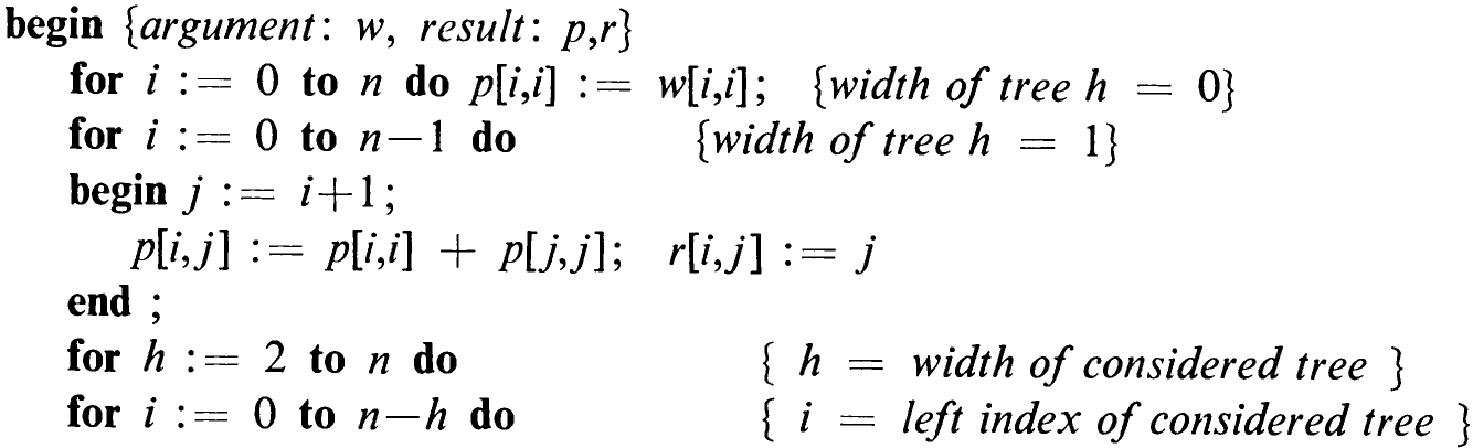
Note that i denotes the left index limit and j the right index limit in the considered tree 7;;. For the cases h > 1 we use a repetitive statement with h ranging from 2 to n, the case h = n spanning the entire tree 7, ,,. In each case the minimal path length p,, and the associated root index r;; are determined by a simple repetitive statement with an index k ranging over the interval given by (4.73).

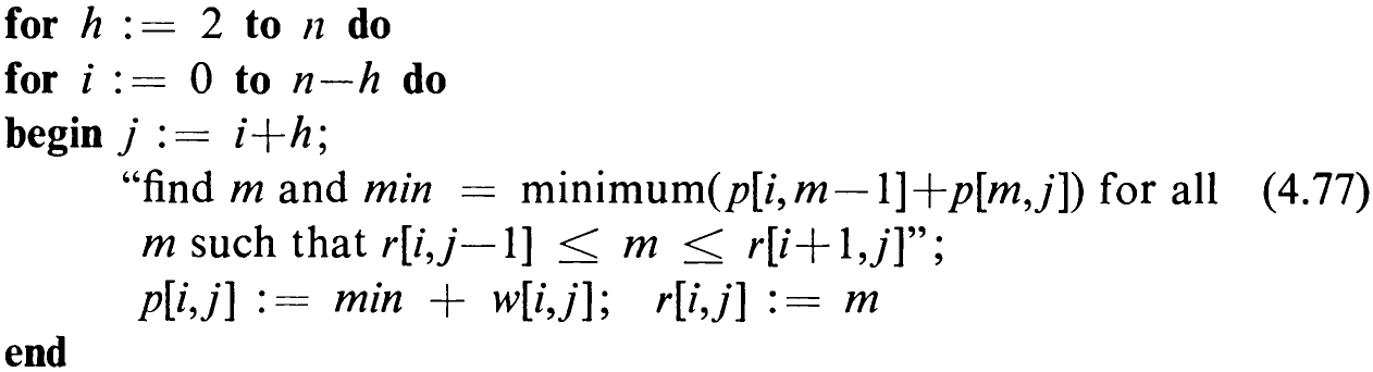
The details of the refinement of the statement within quotes can be found in Program 4.6. The average path length of T,,, is now given by the quotient Po,nlWo,, and its root is the node with index ry,,.

It is evident from algorithm (4.77) that the effort to determine the optimal structure is of the order O(n?); also, the amount of required storage is O(n’). This is unacceptable if ” is very large. Algorithms with greater efficiency are therefore highly desirable. One of them is the algorithm developed by Hu and Tucker [4-5] which requires only O(n) storage and O(n-log n) computations. However, it considers only the case in which the key frequencies are zero (a; = 0), i.e., where only the unsuccessful search trials are registered. Another algorithm, also requiring O(m) storage elements and O(u- log m) computations was described by Walker and Gotlieb [4-11]. Instead of trying to find the optimum, this algorithm merely promises to yield a nearly optimal tree. It can therefore be based on heuristic principles. The basic idea is the following.

Consider the nodes (true and special nodes) being distributed on a linear scale, weighted by their frequencies (or probabilities) of access. Then find the node which is closest to the “center of gravity.” This node is called the centroid, and its index is

rounded to the nearest integer. If all nodes have equal weight, then the root of the desired optimal tree evidently coincides with the centroid, and—so the reasoning goes—it will in most cases be in the close neighborhood of the centroid. A limited search is then used to find the local optimum, whereafter232 this procedure is applied to the resulting two subtrees. The likelihood of the root lying very close to the centroid grows with the size n of the tree. As soon as the subtrees have reached a “manageable” size, their optimum can be determined by the above exact algorithm.

4.4.10 Displaying a Tree Structure

We now turn to the associated programming problem of how to generate an output which displays the structure of the tree in a reasonably clear, graphic form, given only the means of the ordinary printer. That is, we should like to draw a picture of the tree, printing the keys as nodes and connecting them with appropriate horizontal and vertical bar characters.

On a line printer whose data we represent as a textfile, i.e., as a sequence of characters, we can proceed only in strict sequence from left to right and from top to bottom. Hence, it seems to be a reasonable idea to first build a representation of the tree that closely reflects its topological structure. The second step then is to map this picture in orderly fashion onto the printed page and to compute the precise coordinates of the nodes and arcs.

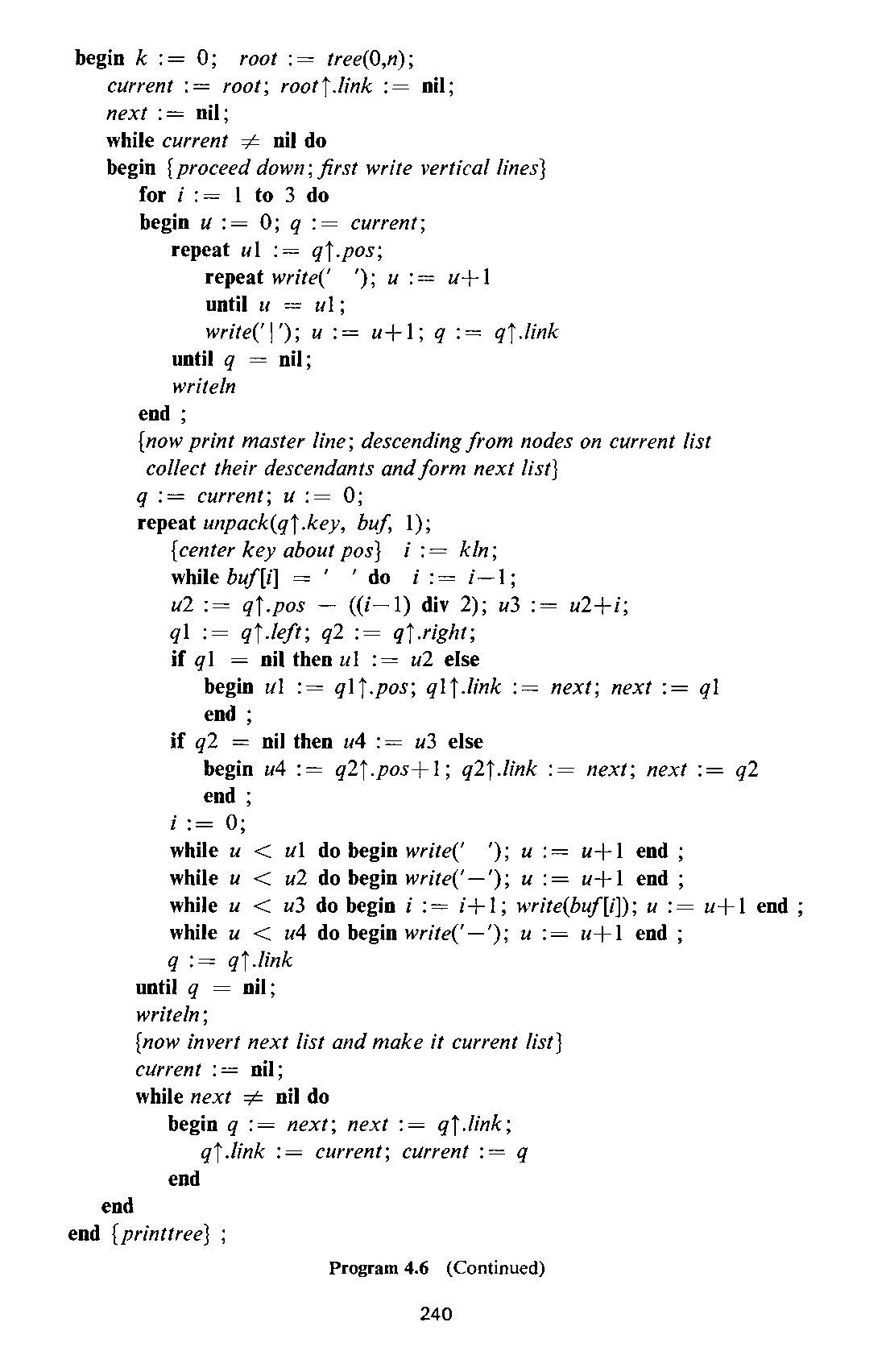
For the first task we can readily draw on our experience with tree generating algorithms and unhesitatingly we adopt a recursive solution to the recursively defined problem. We formulate a function procedure called tree similar to the one used in Program 4.3. The parameters i and j are the limiting indices of the nodes belonging to the tree. Its root is then defined as the node with index r;;. Before proceeding, however, we need to define the type of the variables that are to represent the nodes. They must contain the two pointers to their subtrees and the key of the node. For purposes to be discussed in the second step, two additional fields, called pos and link, are also incorporated. The chosen definitions are shown in (4.79) and the resulting function procedure is listed in Program 4.6.

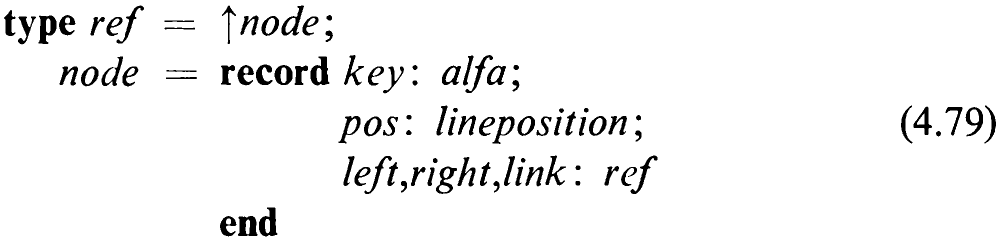
Note that this procedure counts the number of generated nodes by the global counter variable k. The kth node is assigned the kth key, and as the keys are alphabetically ordered, k multiplied by a constant scale factor yields the horizontal coordinate of each key, a value which is immediately stored along with the other information. Note also that we have departed from the convention of using integers as keys, and we assume them to be of a type alfa, standing for an array of characters of a given (maximum) length upon which alphabetical ordering is defined.

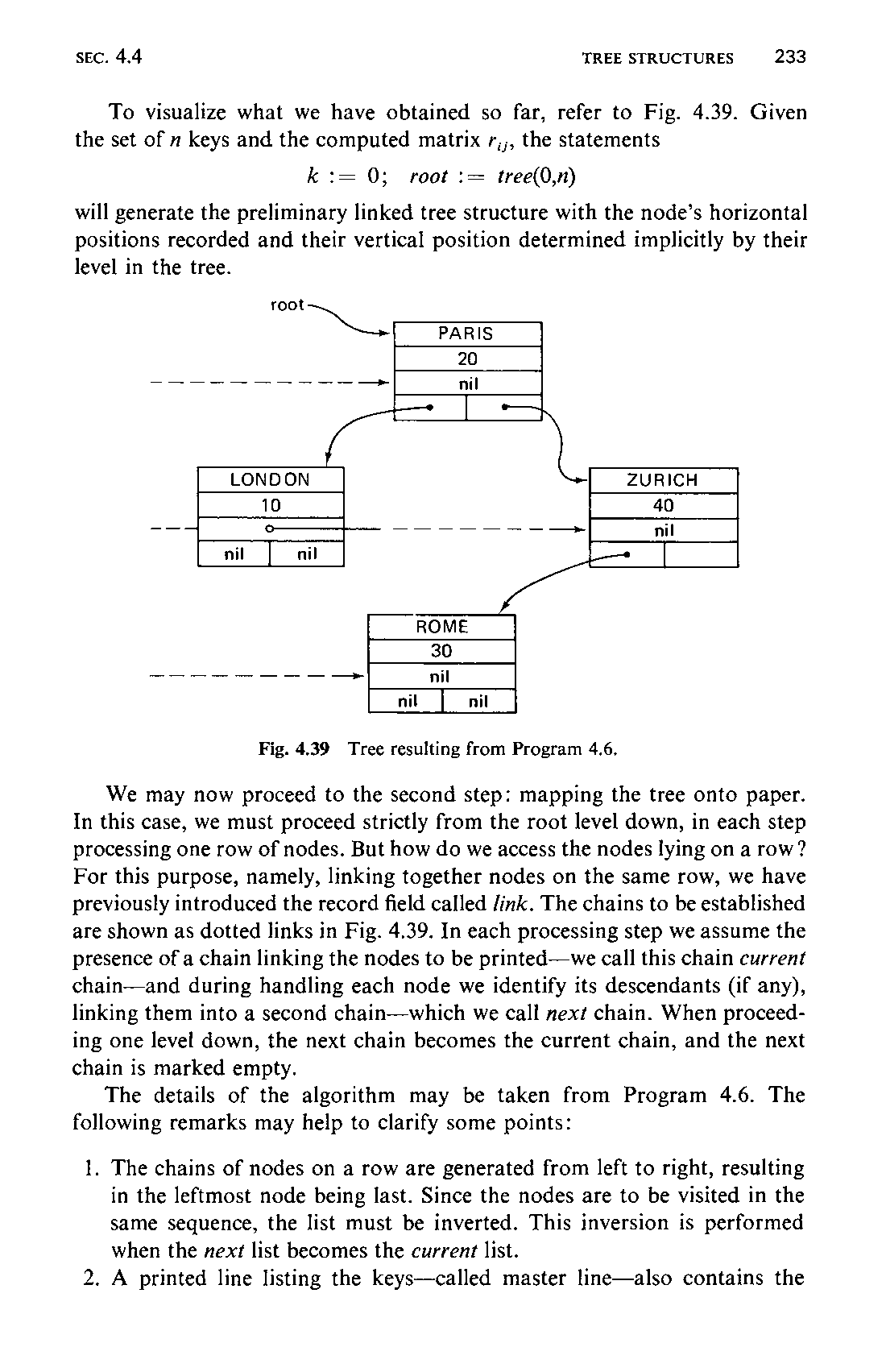
To visualize what we have obtained so far, refer to Fig. 4.39. Given the set of n keys and the computed matrix r,,, the statements

will generate the preliminary linked tree structure with the node’s horizontal positions recorded and their vertical position determined implicitly by their level in the tree.

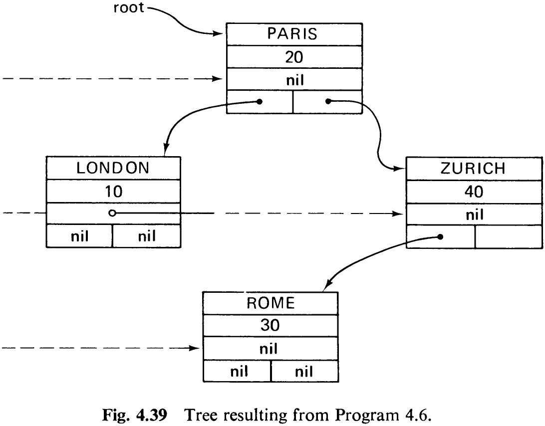
We may now proceed to the second step: mapping the tree onto paper. In this case, we must proceed strictly from the root level down, in each step processing one row of nodes. But how do we access the nodes lying on a row? For this purpose, namely, linking together nodes on the same row, we have previously introduced the record field called link. The chains to be established are shown as dotted links in Fig. 4.39. In each processing step we assume the presence of a chain linking the nodes to be printed—we call this chain current chain—and during handling each node we identify its descendants (if any), linking them into a second chain—which we call next chain. When proceeding one level down, the next chain becomes the current chain, and the next chain is marked empty.

The details of the algorithm may be taken from Program 4.6. The following remarks may help to clarify some points:

1. The chains of nodes on a row are generated from left to right, resulting in the leftmost node being last. Since the nodes are to be visited in the same sequence, the list must be inverted. This inversion is performed when the next list becomes the current list.

2. A printed line listing the keys—called master line—also contains the

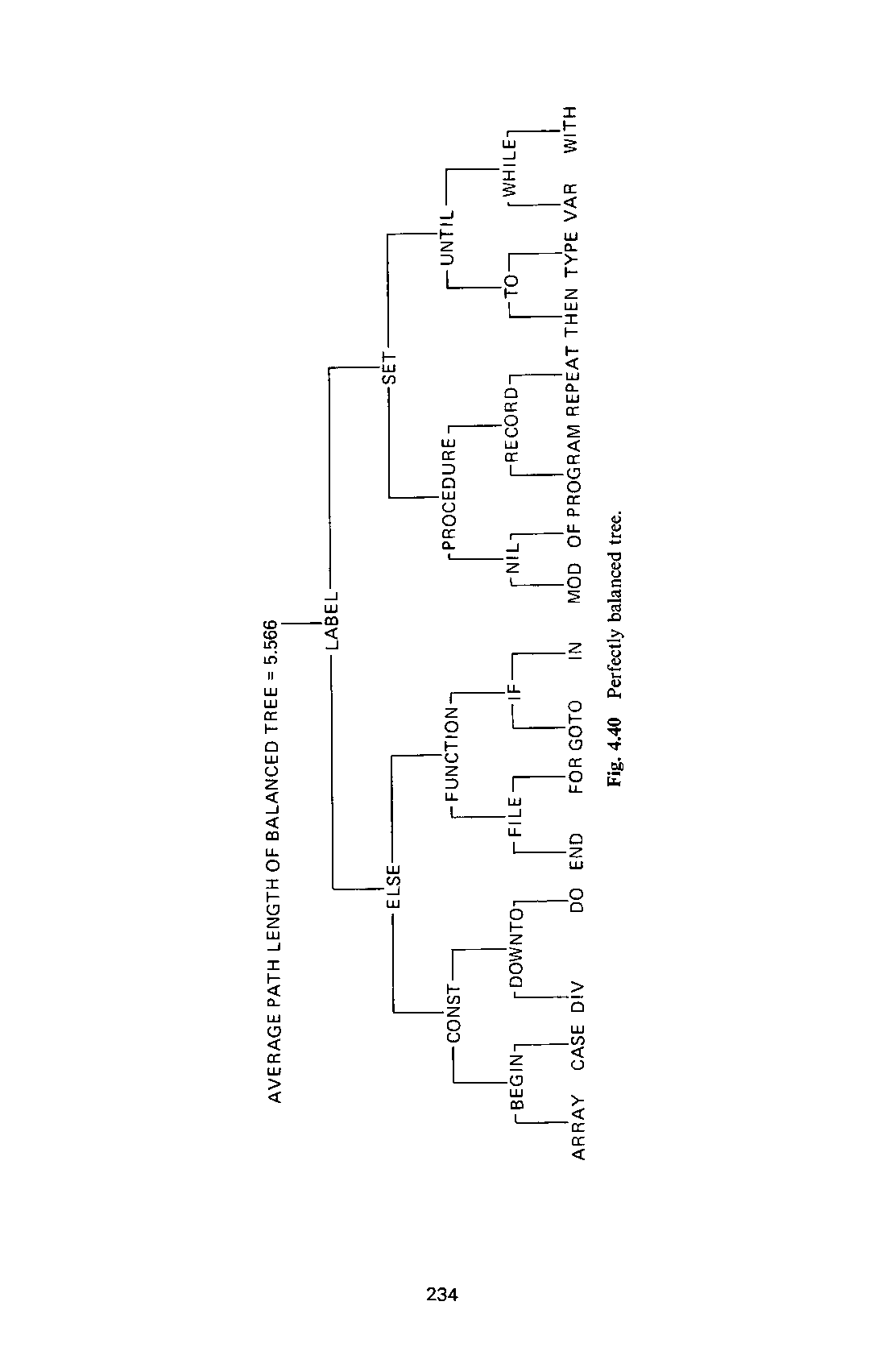
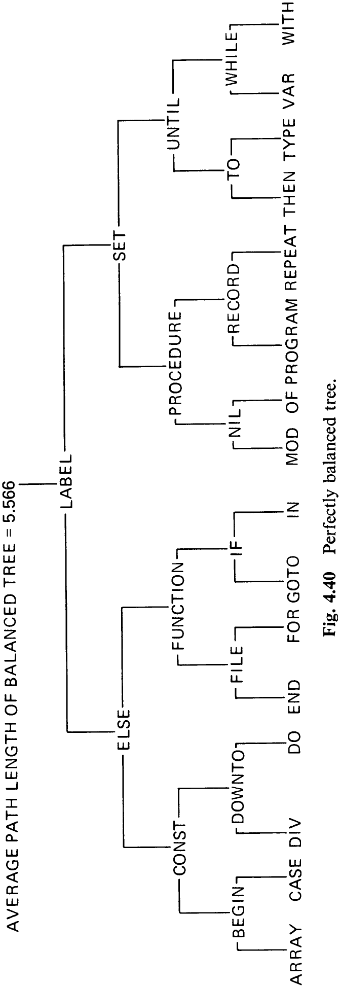
horizontal arcs (see Fig. 4.40). The variables w1, v2, u3, u4 denote the beginning and end positions of the left and right horizontal arcs of a node.

3. The construction of each master line is preceded by three lines for marking the vertical parts of the arcs.

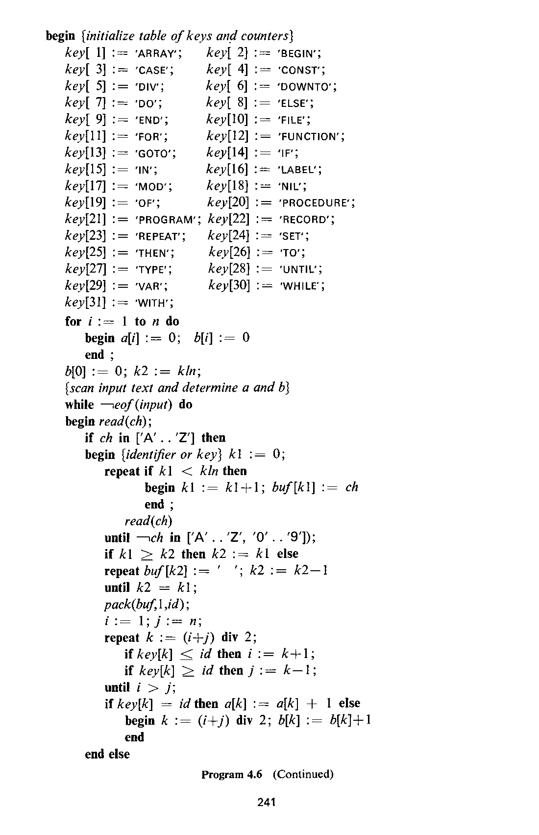
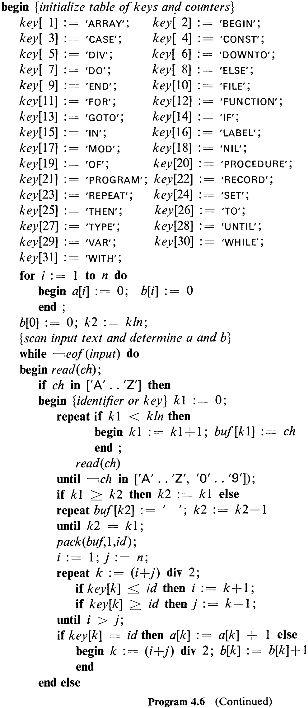
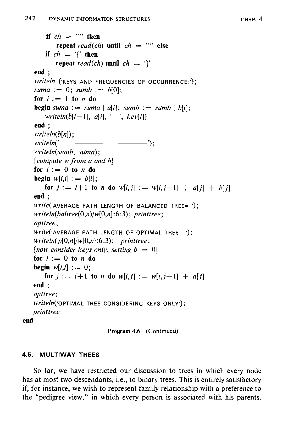
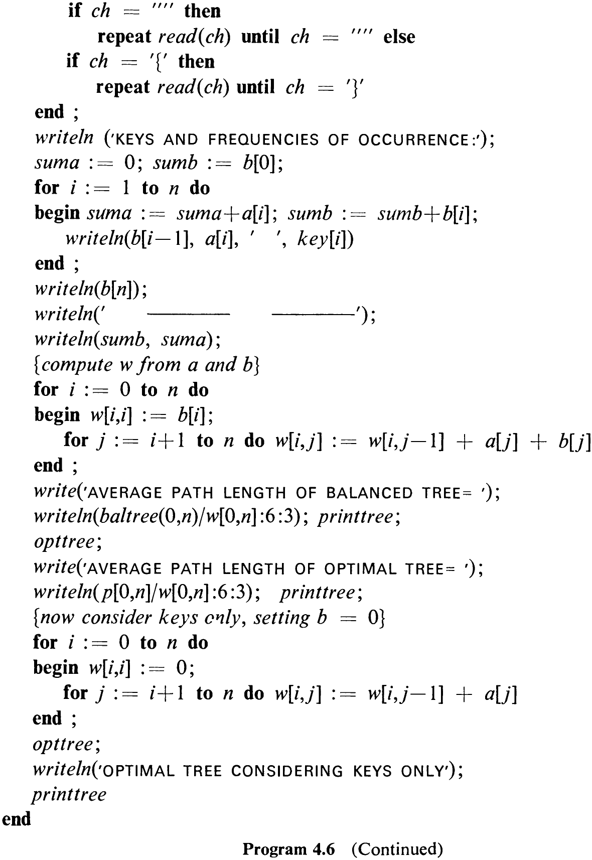
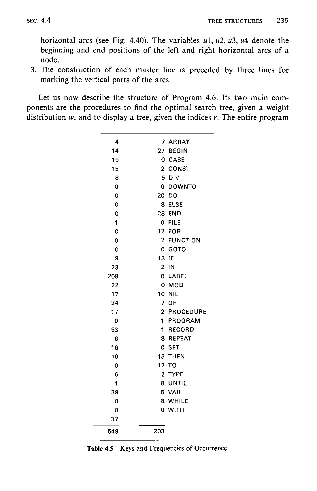
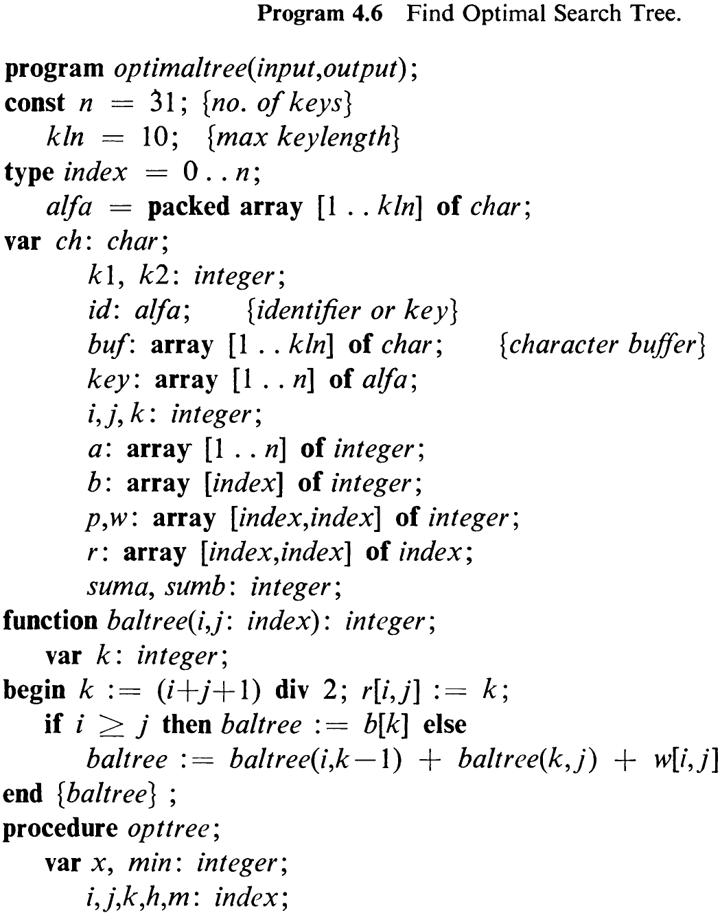
Let us now describe the structure of Program 4.6. Its two main components are the procedures to find the optimal search tree, given a weight distribution w, and to display a tree, given the indices r. The entire program

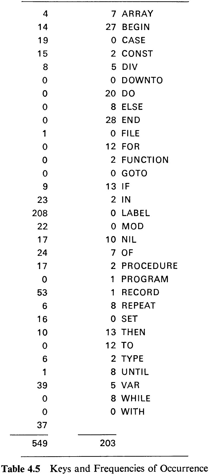
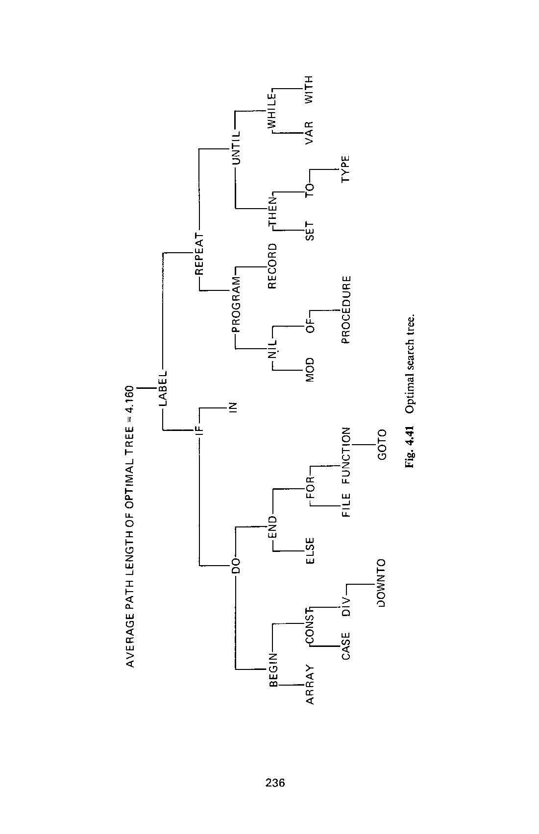
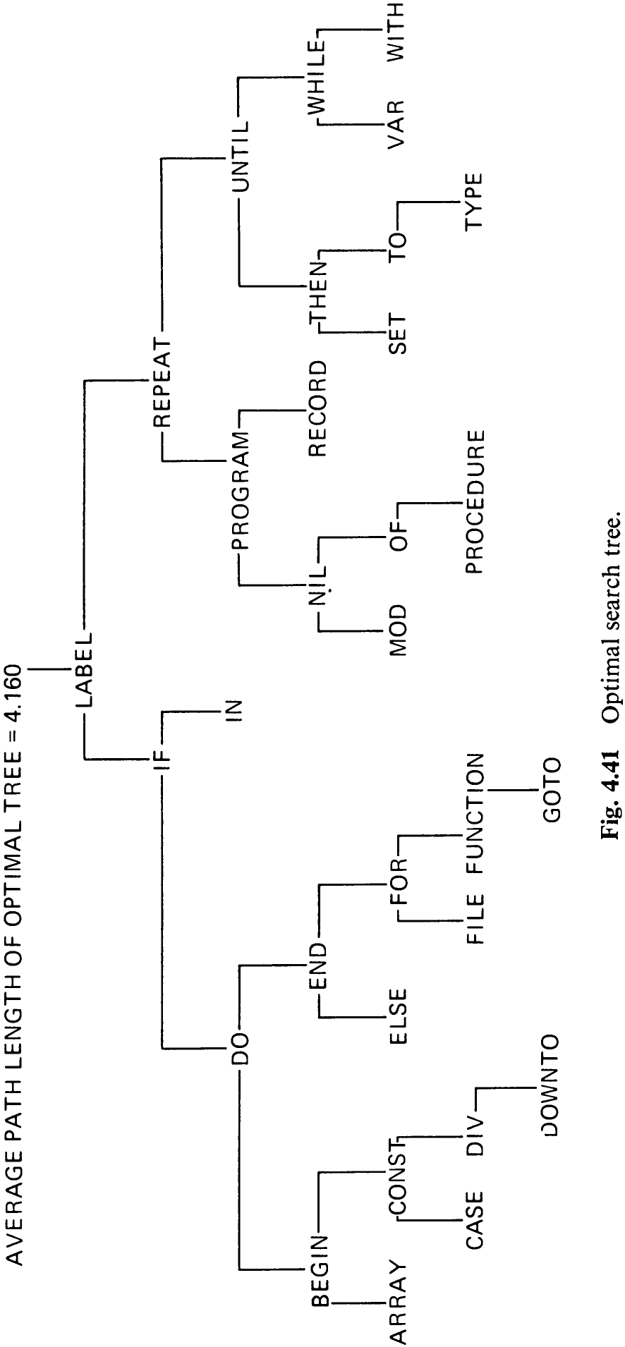
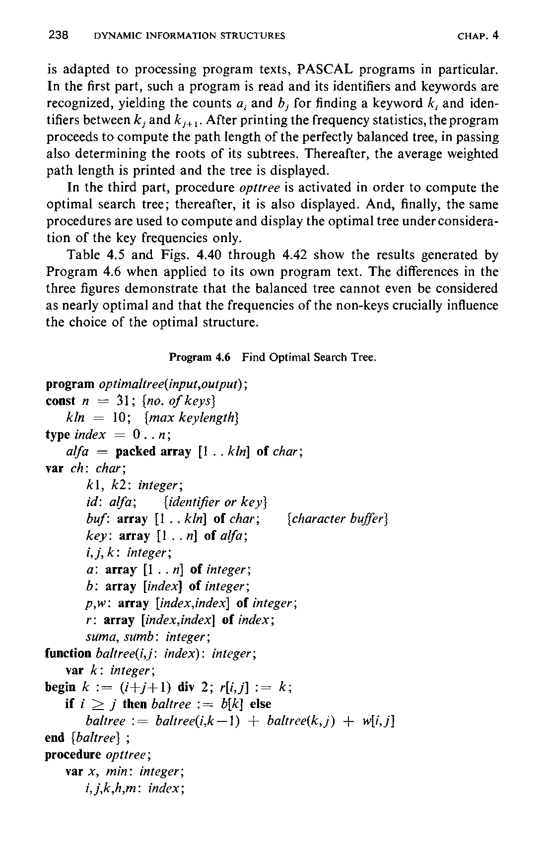
is adapted to processing program texts, PASCAL programs in particular. In the first part, such a program is read and its identifiers and keywords are recognized, yielding the counts a, and 5, for finding a keyword k, and identifiers between k,; and k,,,. After printing the frequency statistics, the program proceeds to compute the path length of the perfectly balanced tree, in passing also determining the roots of its subtrees. Thereafter, the average weighted path length is printed and the tree is displayed.

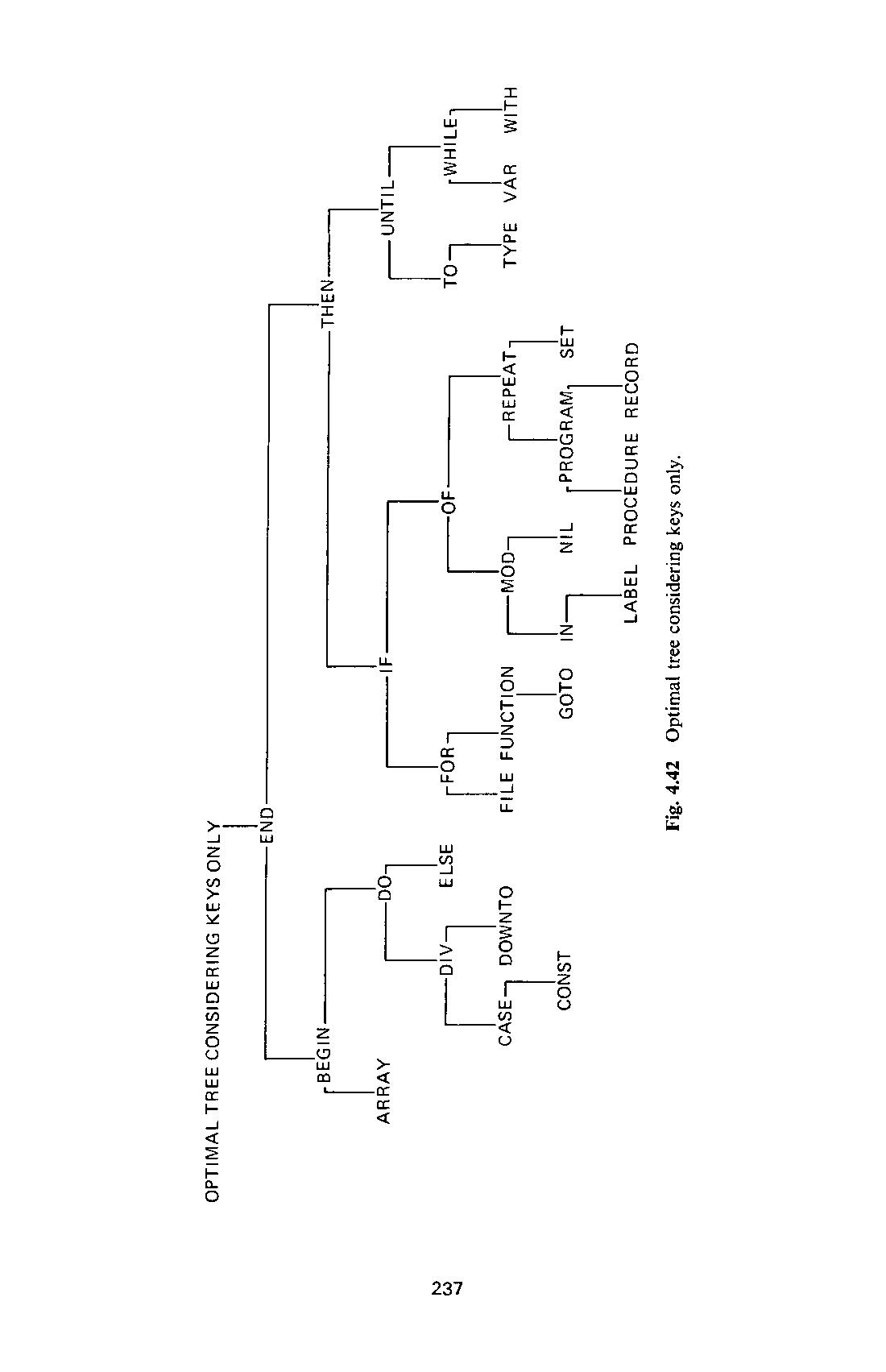
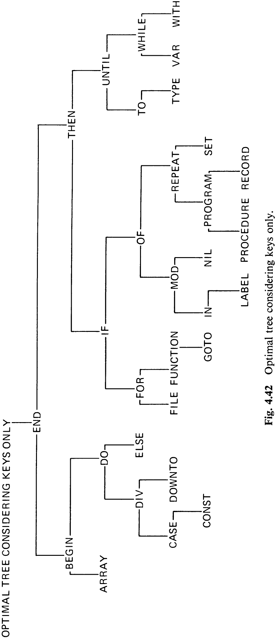
In the third part, procedure opttree is activated in order to compute the optimal search tree; thereafter, it is also displayed. And, finally, the same procedures are used to compute and display the optimal tree under consideration of the key frequencies only.

Table 4.5 and Figs. 4.40 through 4.42 show the results generated by Program 4.6 when applied to its own program text. The differences in the three figures demonstrate that the balanced tree cannot even be considered as nearly optimal and that the frequencies of the non-keys crucially influence the choice of the optimal structure.

begin j := i+h; { j = right index of considered tree }