Multiway Trees

So far, we have restricted our discussion to trees in which every node has at most two descendants, i.e., to binary trees. This is entirely satisfactory if, for instance, we wish to represent family relationship with a preference to the “pedigree view,” in which every person is associated with his parents.243 After all, no one has more than two parents! But what about someone who prefers the “posterity view” ? He has to cope with the fact that some people have more than two children, and his trees will contain nodes with many branches. For lack of a better term, we shall call them multiway trees.

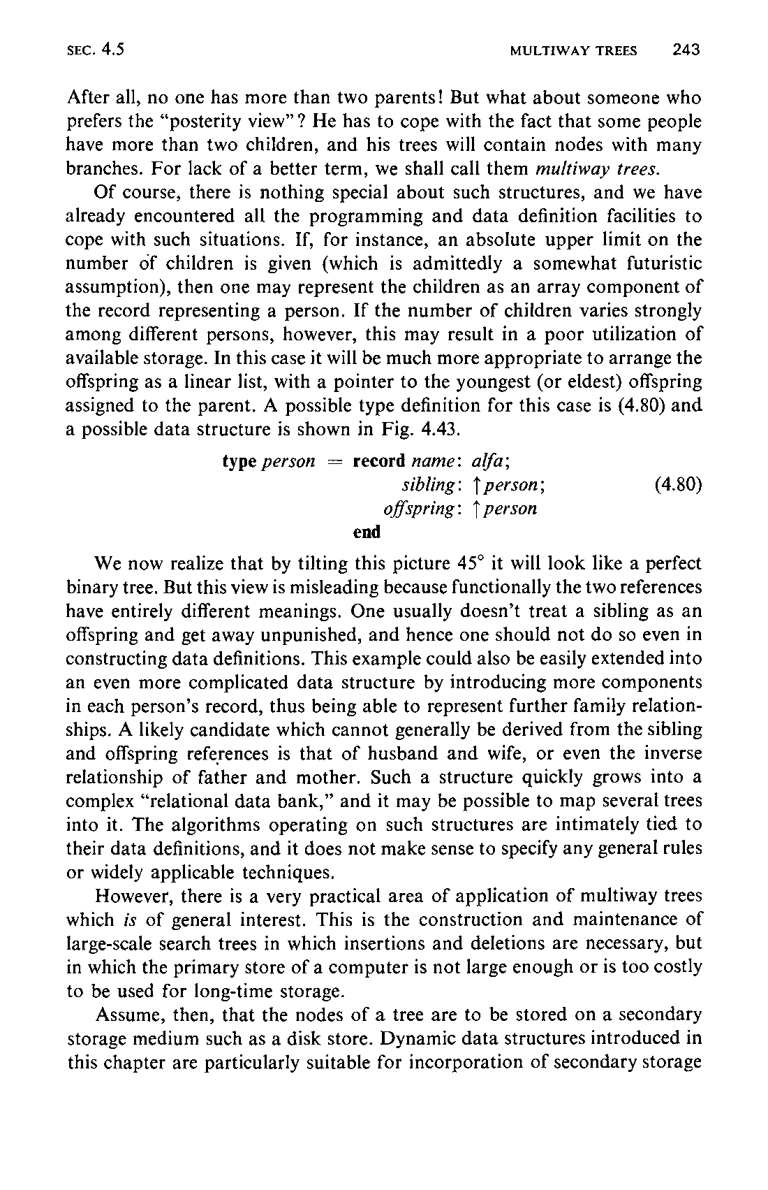
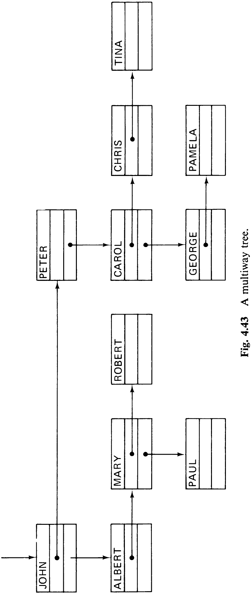
Of course, there is nothing special about such structures, and we have already encountered all the programming and data definition facilities to cope with such situations. If, for instance, an absolute upper limit on the number of children is given (which is admittedly a somewhat futuristic assumption), then one may represent the children as an array component of the record representing a person. If the number of children varies strongly among different persons, however, this may result in a poor utilization of available storage. In this case it will be much more appropriate to arrange the offspring as a linear list, with a pointer to the youngest (or eldest) offspring assigned to the parent. A possible type definition for this case is (4.80) and a possible data structure is shown in Fig. 4.43.

We now realize that by tilting this picture 45° it will look like a perfect binary tree. But this view is misleading because functionally the two references have entirely different meanings. One usually doesn’t treat a sibling as an offspring and get away unpunished, and hence one should not do so even in constructing data definitions. This example could also be easily extended into an even more complicated data structure by introducing more components in each person’s record, thus being able to represent further family relationships. A likely candidate which cannot generally be derived from the sibling and offspring references is that of husband and wife, or even the inverse relationship of father and mother. Such a structure quickly grows into a complex “relational data bank,” and it may be possible to map several trees into it. The algorithms operating on such structures are intimately tied to their data definitions, and it does not make sense to specify any general rules or widely applicable techniques.

However, there is a very practical area of application of multiway trees which is of general interest. This is the construction and maintenance of large-scale search trees in which insertions and deletions are necessary, but in which the primary store of a computer is not large enough or is too costly to be used for long-time storage.

Assume, then, that the nodes of a tree are to be stored on a secondary storage medium such as a disk store. Dynamic data structures introduced in this chapter are particularly suitable for incorporation of secondary storage

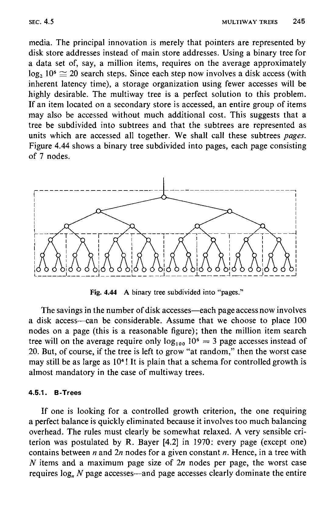
media. The principal innovation is merely that pointers are represented by disk store addresses instead of main store addresses. Using a binary tree for a data set of, say, a million items, requires on the average approximately log, 10° = 20 search steps. Since each step now involves a disk access (with inherent latency time), a storage organization using fewer accesses will be highly desirable. The multiway tree is a perfect solution to this problem. If an item located on a secondary store is accessed, an entire group of items may also be accessed without much additional cost. This suggests that a tree be subdivided into subtrees and that the subtrees are represented as units which are accessed all together. We shall call these subtrees pages. Figure 4.44 shows a binary tree subdivided into pages, each page consisting of 7 nodes.

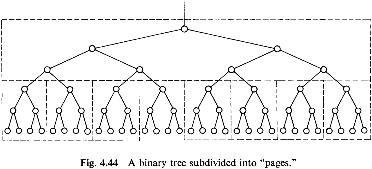
The savings in the number of disk accesses—each page access now involves a disk access—can be considerable. Assume that we choose to place 100 nodes on a page (this is a reasonable figure); then the million item search tree will on the average require only log,,, 10° = 3 page accesses instead of 20. But, of course, if the tree is left to grow “at random,” then the worst case may still be as large as 10*! It is plain that a schema for controlled growth is almost mandatory in the case of multiway trees.

4.5.1 B-Trees

If one is looking for a controlled growth criterion, the one requiring a perfect balance is quickly eliminated because it involves too much balancing overhead. The rules must clearly be somewhat relaxed. A very sensible criterion was postulated by R. Bayer [4.2] in 1970: every page (except one) contains between n and 2n nodes for a given constant n. Hence, in a tree with N items and a maximum page size of 2n nodes per page, the worst case requires log, N page accesses—and page accesses clearly dominate the entire246 search effort. Moreover, the important factor of store utilization is at least 50% since pages are always at least half full. With all these advantages, the schema involves comparatively simple algorithms for search, insertion, and deletion. We will subsequently study them in detail.

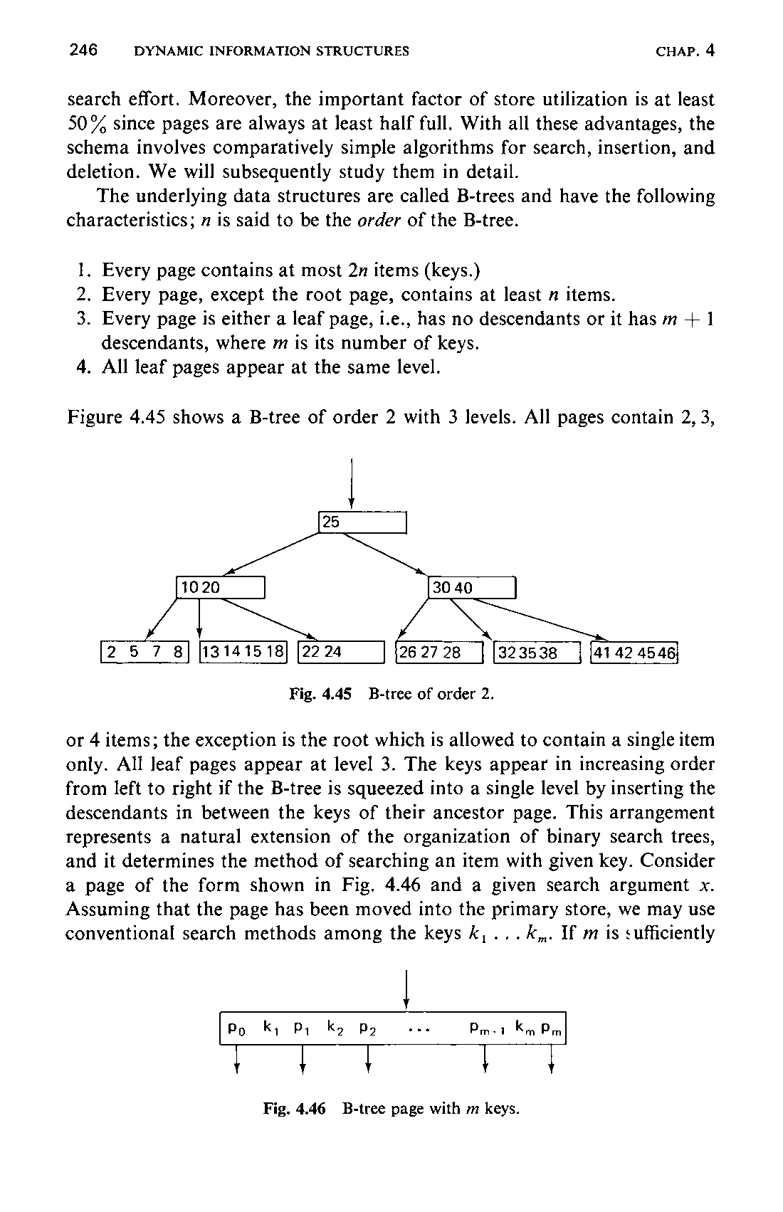
The underlying data structures are called B-trees and have the following characteristics; 7 is said to be the order of the B-tree.

1. Every page contains at most 2” items (keys.)

2. Every page, except the root page, contains at least n items.

3. Every page is either a leaf page, i.e., has no descendants or it has m + 1 descendants, where m is its number of keys.

4. All leaf pages appear at the same level.

Figure 4.45 shows a B-tree of order 2 with 3 levels. All pages contain 2, 3,

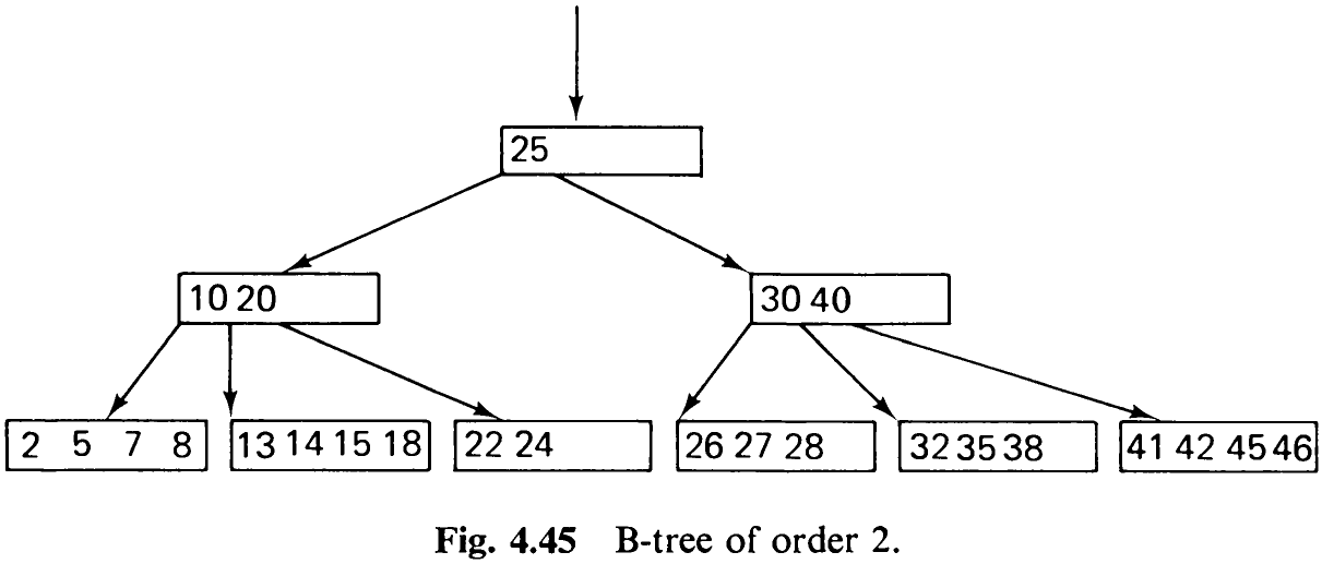
or 4 items; the exception is the root which is allowed to contain a single item only. All leaf pages appear at level 3. The keys appear in increasing order from left to right if the B-tree is squeezed into a single level by inserting the descendants in between the keys of their ancestor page. This arrangement represents a natural extension of the organization of binary search trees, and it determines the method of searching an item with given key. Consider a page of the form shown in Fig. 4.46 and a given search argument x. Assuming that the page has been moved into the primary store, we may use conventional search methods among the keys k, ...k,,. If m is sufficiently

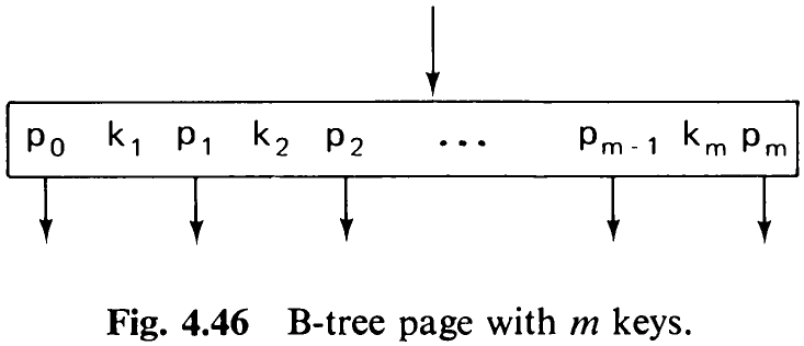
large, one may use binary search; if it is rather small, an ordinary sequential search will do. (Note that the time required for a search in main store is probably negligible compared to the time it takes to move the page from secondary into primary store.) If the search is unsuccessful, we are in one of the following situations:

2. Ki, <x. The search continues on page p,,}.

3. x < k,. The search continues on page po}.

If in some case the designated pointer is nil, i.e., if there is no descendant page, then there is no item with key x in the whole tree, and the search is terminated.

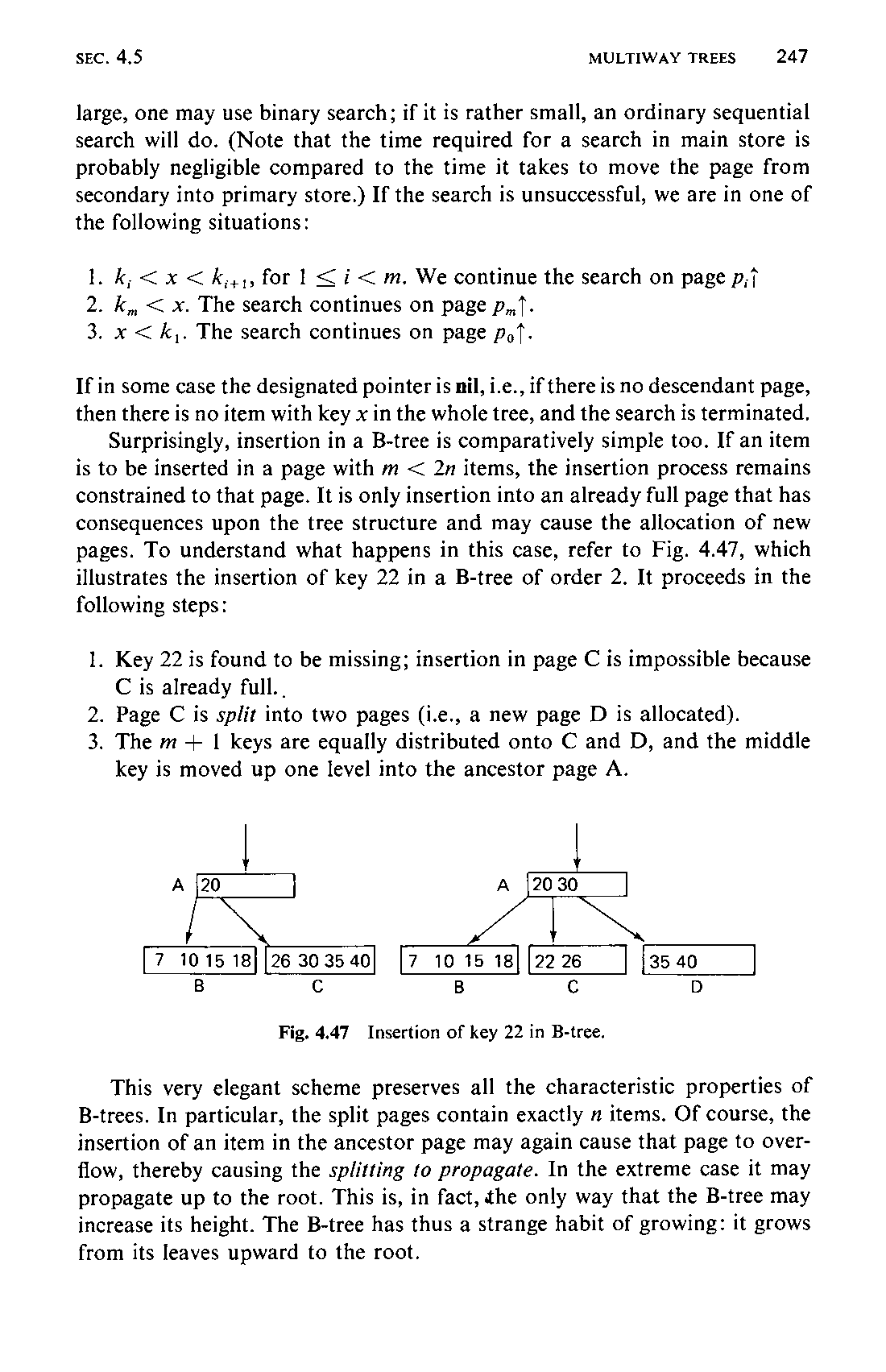
Surprisingly, insertion in a B-tree is comparatively simple too. If an item is to be inserted in a page with m < 2n items, the insertion process remains constrained to that page. It is only insertion into an already full page that has consequences upon the tree structure and may cause the allocation of new pages. To understand what happens in this case, refer to Fig. 4.47, which illustrates the insertion of key 22 in a B-tree of order 2. It proceeds in the following steps:

1. Key 22 is found to be missing; insertion in page C is impossible because C is already full.

2. Page C is split into two pages (i.e., a new page D is allocated).

3. The m + 1 keys are equally distributed onto C and D, and the middle key is moved up one level into the ancestor page A.

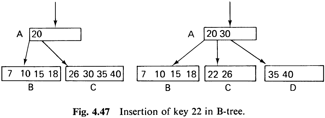
This very elegant scheme preserves all the characteristic properties of B-trees. In particular, the split pages contain exactly n items. Of course, the insertion of an item in the ancestor page may again cause that page to overflow, thereby causing the splitting to propagate. In the extreme case it may propagate up to the root. This is, in fact, the only way that the B-tree may increase its height. The B-tree has thus a strange habit of growing: it grows from its leaves upward to the root.

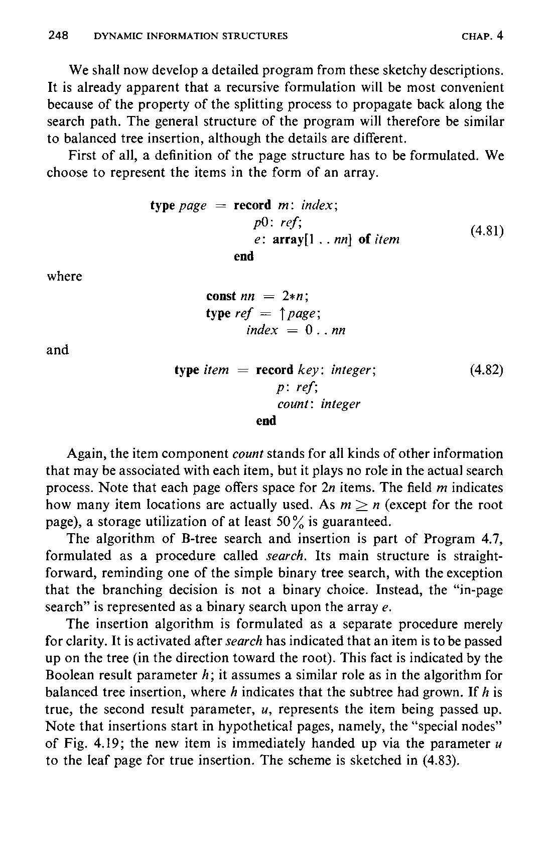
We shall now develop a detailed program from these sketchy descriptions. It is already apparent that a recursive formulation will be most convenient because of the property of the splitting process to propagate back along the search path. The general structure of the program will therefore be similar to balanced tree insertion, although the details are different.

First of all, a definition of the page structure has to be formulated. We choose to represent the items in the form of an array.

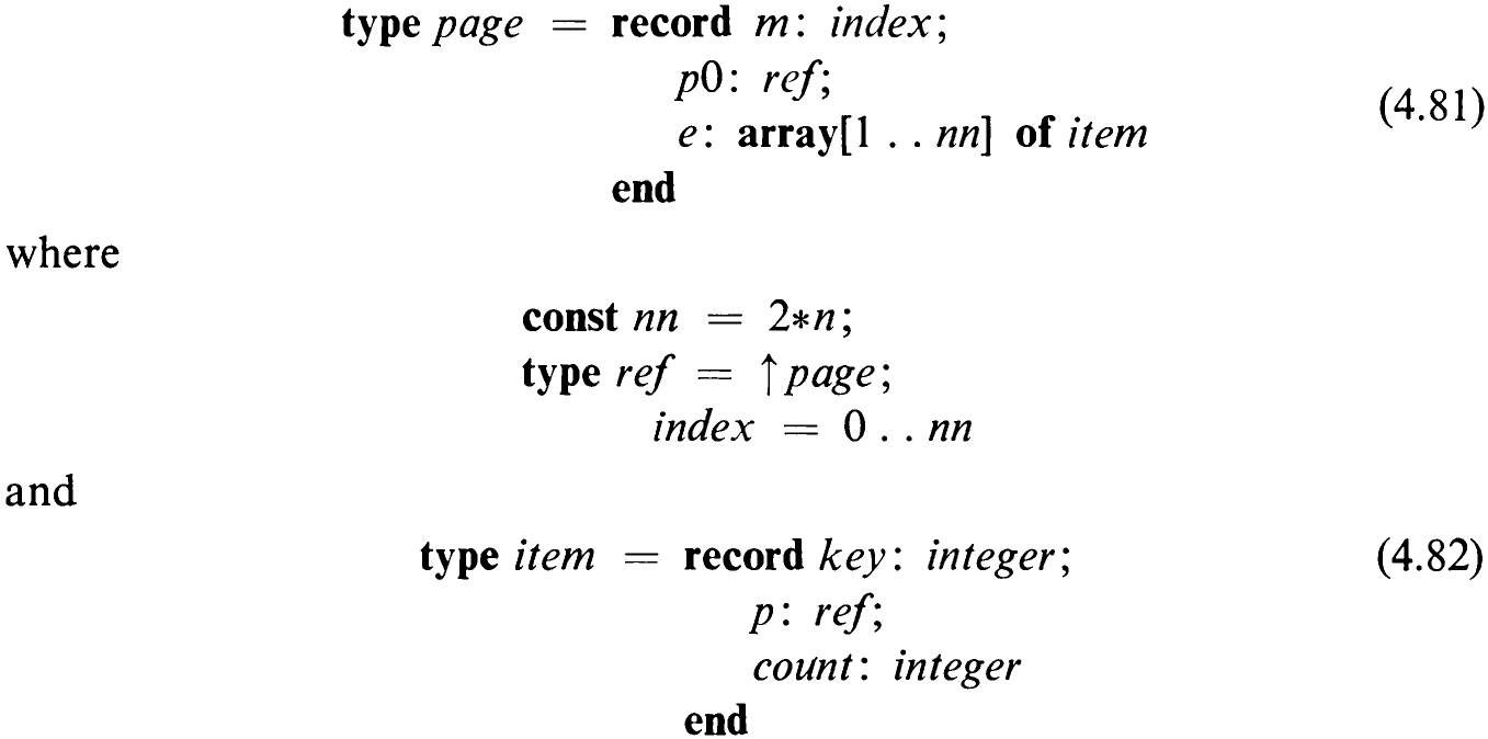
Again, the item component count stands for all kinds of other information that may be associated with each item, but it plays no role in the actual search process. Note that each page offers space for 2 items. The field m indicates how many item locations are actually used. As m > n (except for the root page), a storage utilization of at least 50% is guaranteed.

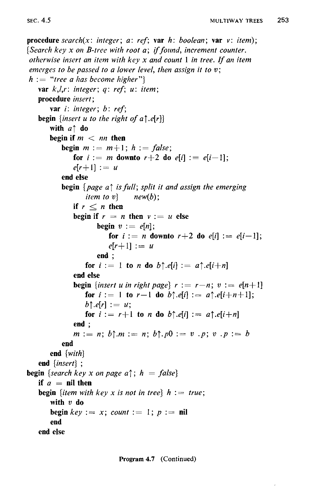
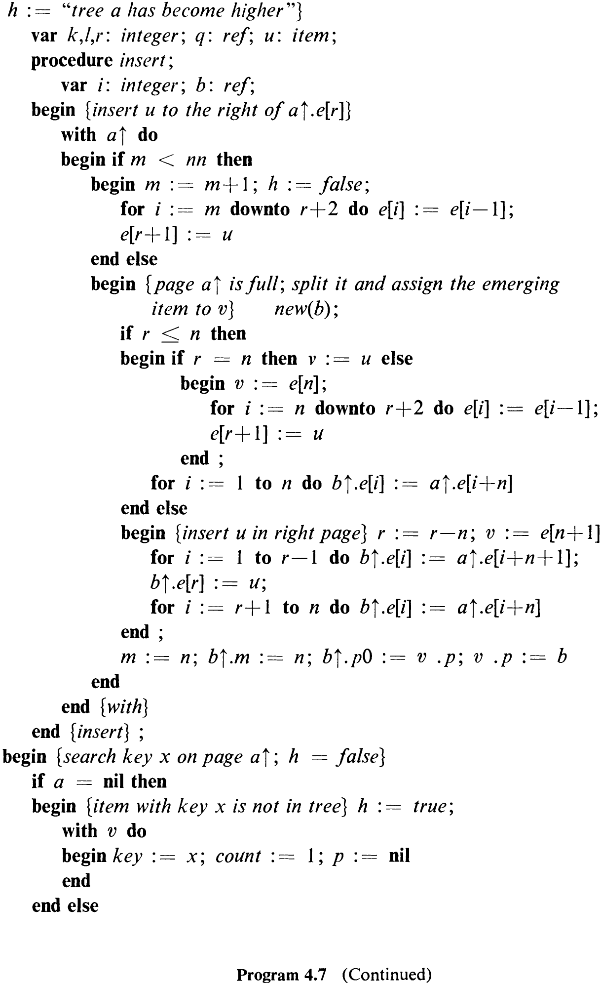
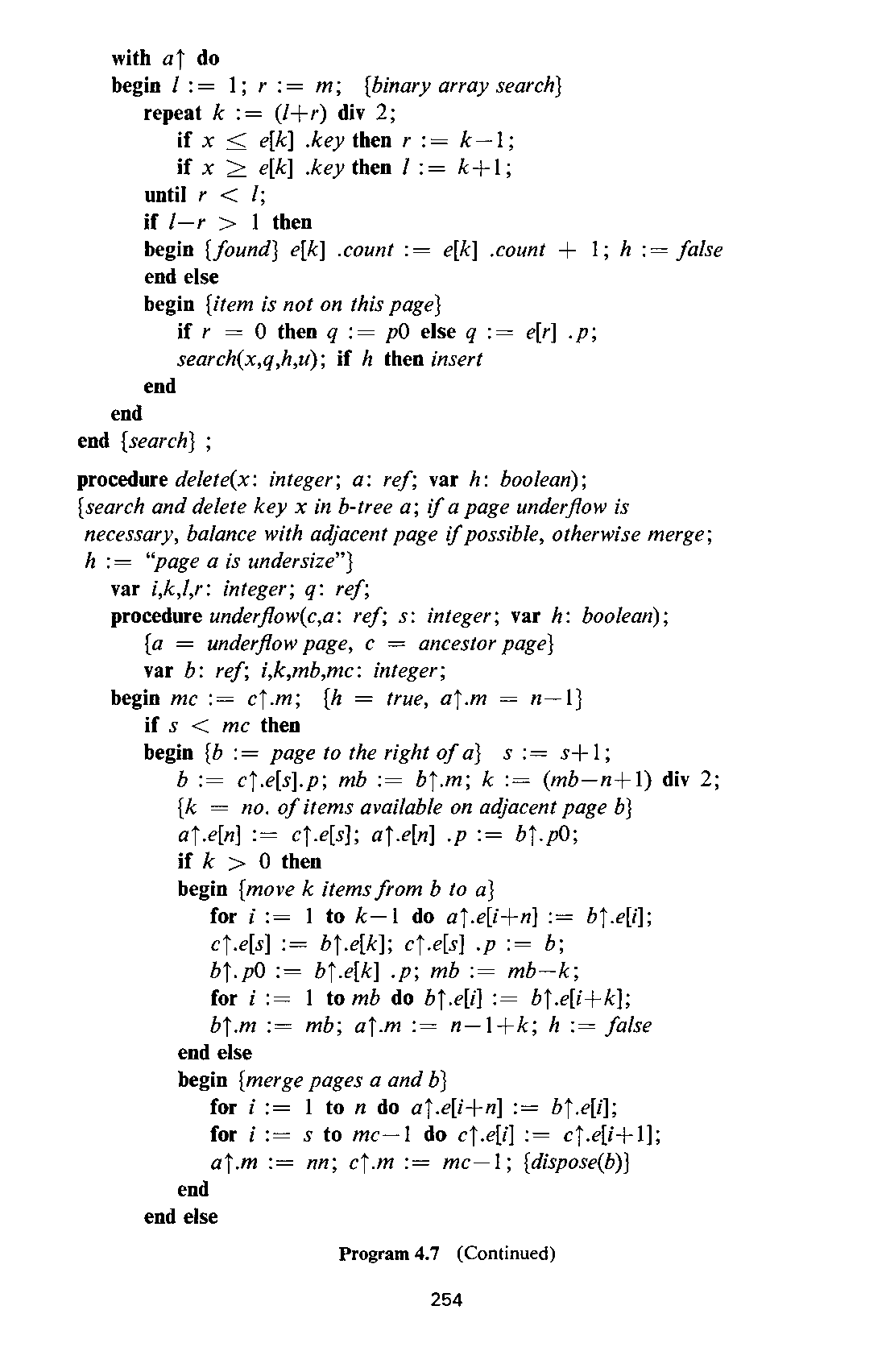
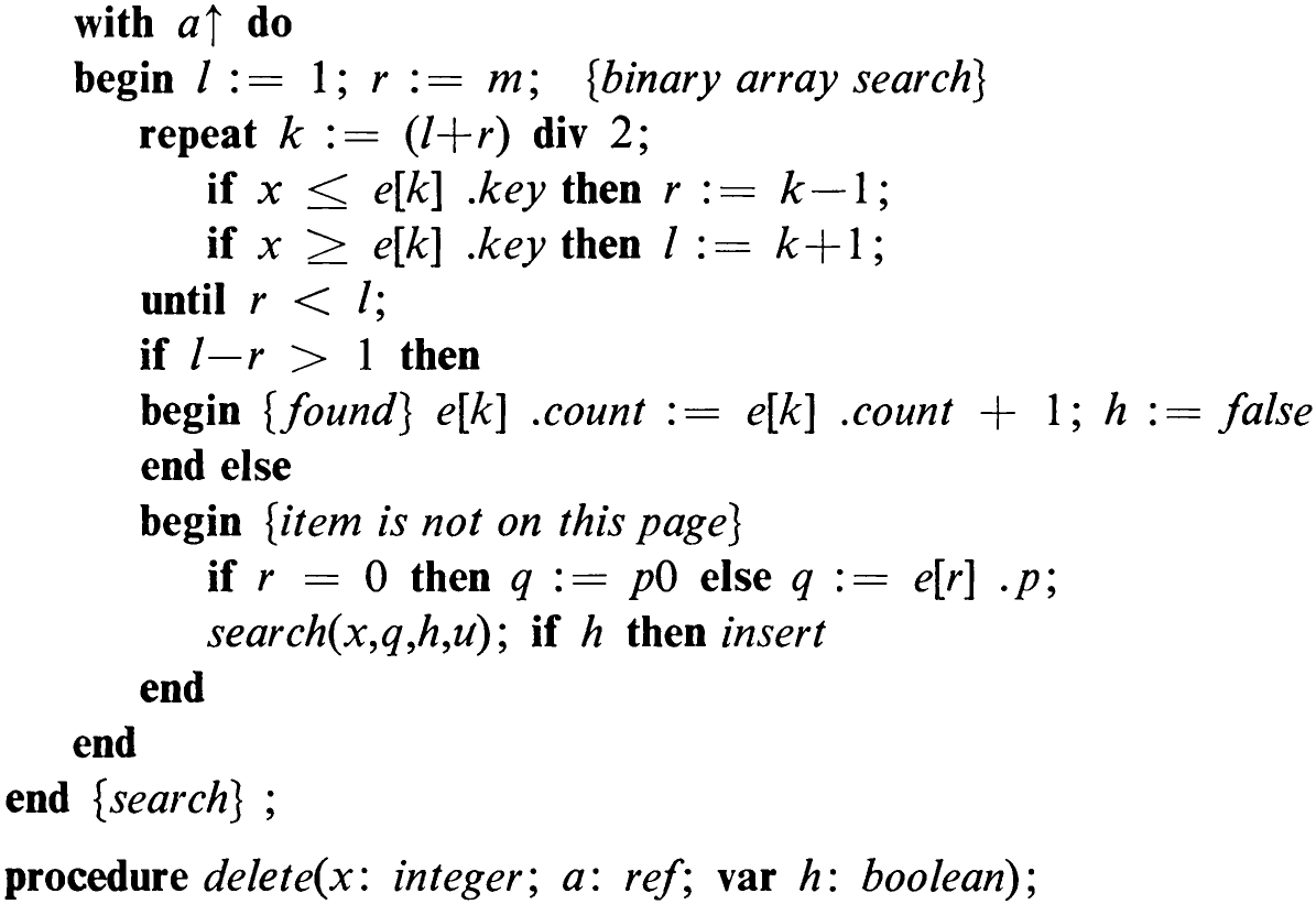
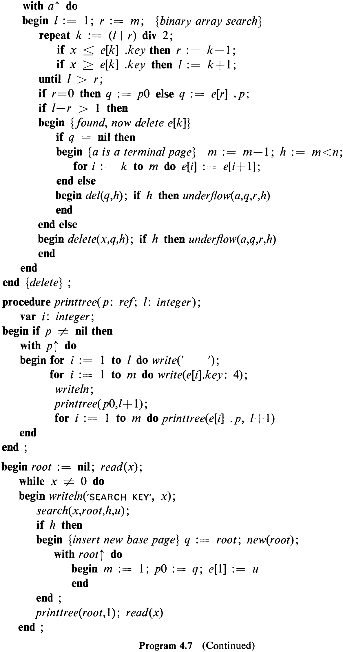
The algorithm of B-tree search and insertion is part of Program 4.7, formulated as a procedure called search. Its main structure is straightforward, reminding one of the simple binary tree search, with the exception that the branching decision is not a binary choice. Instead, the “in-page search” is represented as a binary search upon the array e.

The insertion algorithm is formulated as a separate procedure merely for clarity. It is activated after search has indicated that an item is to be passed up on the tree (in the direction toward the root). This fact is indicated by the Boolean result parameter h; it assumes a similar role as in the algorithm for balanced tree insertion, where / indicates that the subtree had grown. If h is true, the second result parameter, u, represents the item being passed up. Note that insertions start in hypothetical pages, namely, the “special nodes” of Fig. 4.19; the new item is immediately handed up via the parameter u to the leaf page for true insertion. The scheme is sketched in (4.83).

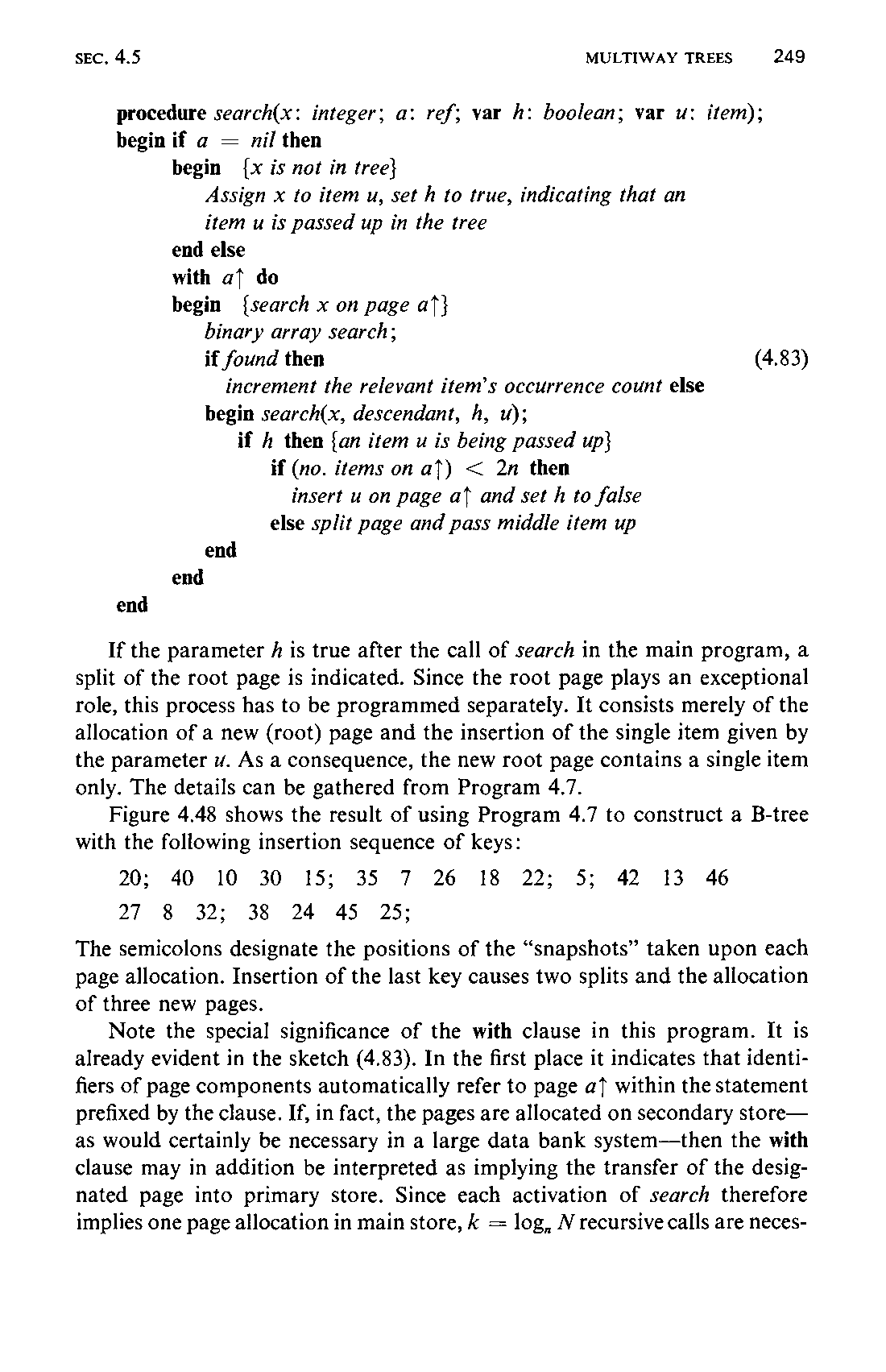
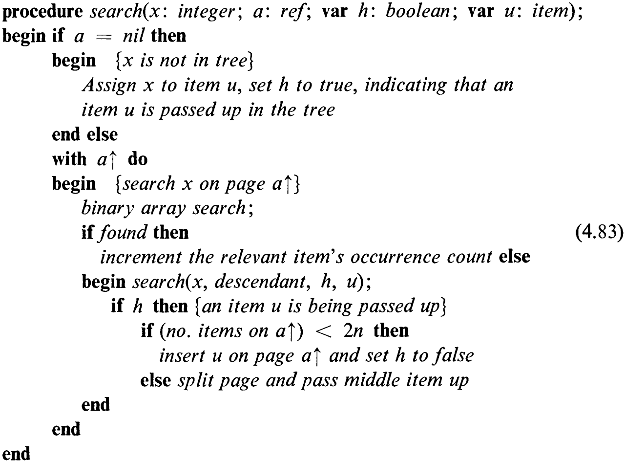
If the parameter A is true after the call of search in the main program, a split of the root page is indicated. Since the root page plays an exceptional role, this process has to be programmed separately. It consists merely of the allocation of a new (root) page and the insertion of the single item given by the parameter uw. As a consequence, the new root page contains a single item only. The details can be gathered from Program 4.7.

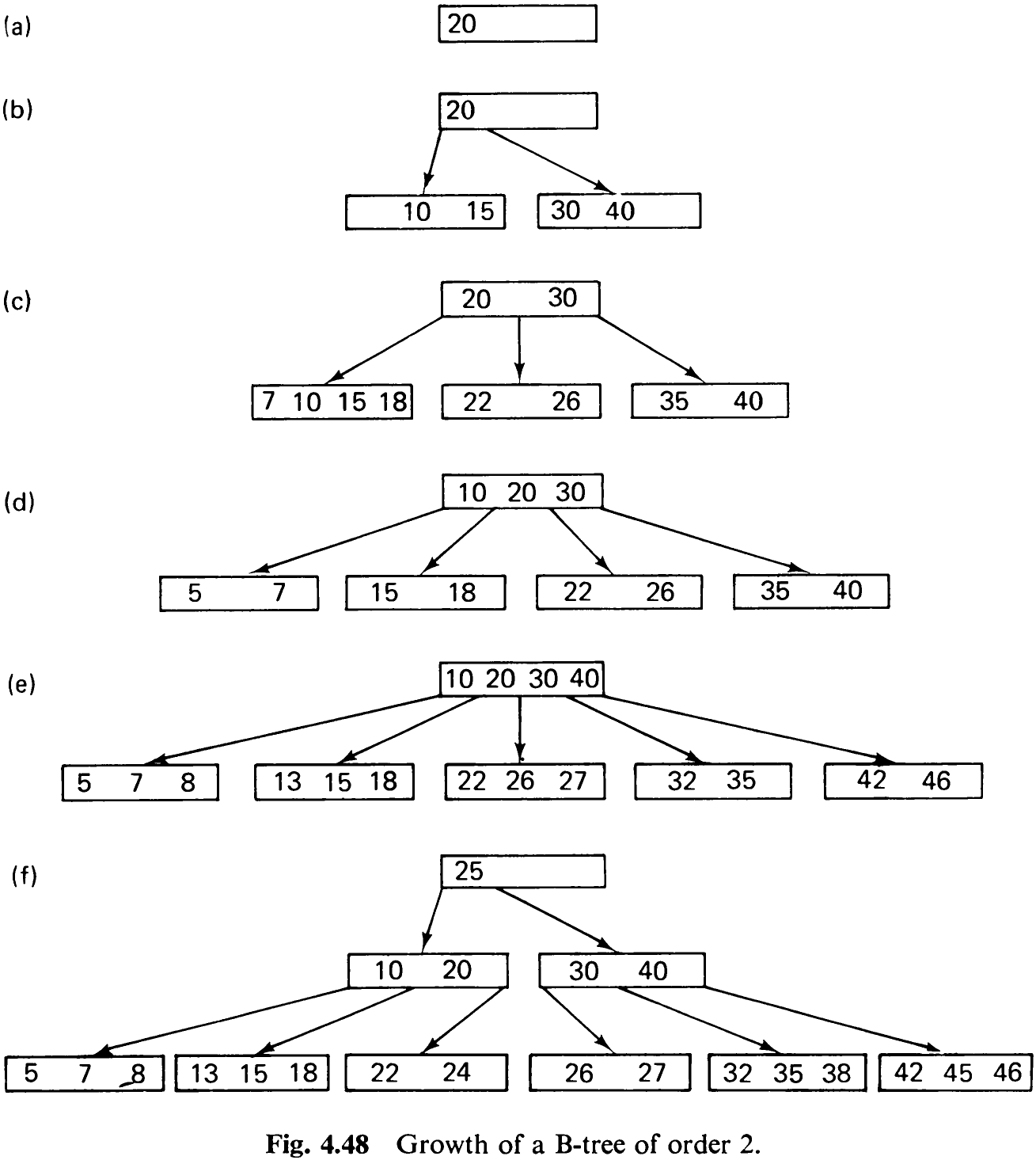
Figure 4.48 shows the result of using Program 4.7 to construct a B-tree with the following insertion sequence of keys:

The semicolons designate the positions of the “snapshots” taken upon each page allocation. Insertion of the last key causes two splits and the allocation of three new pages.

Note the special significance of the with clause in this program. It is already evident in the sketch (4.83). In the first place it indicates that identifiers of page components automatically refer to page a} within the statement prefixed by the clause. If, in fact, the pages are allocated on secondary store—as would certainly be necessary in a large data bank system—then the with clause may in addition be interpreted as implying the transfer of the designated page into primary store. Since each activation of search therefore implies one page allocation in main store, k = log, N recursive calls are neces-

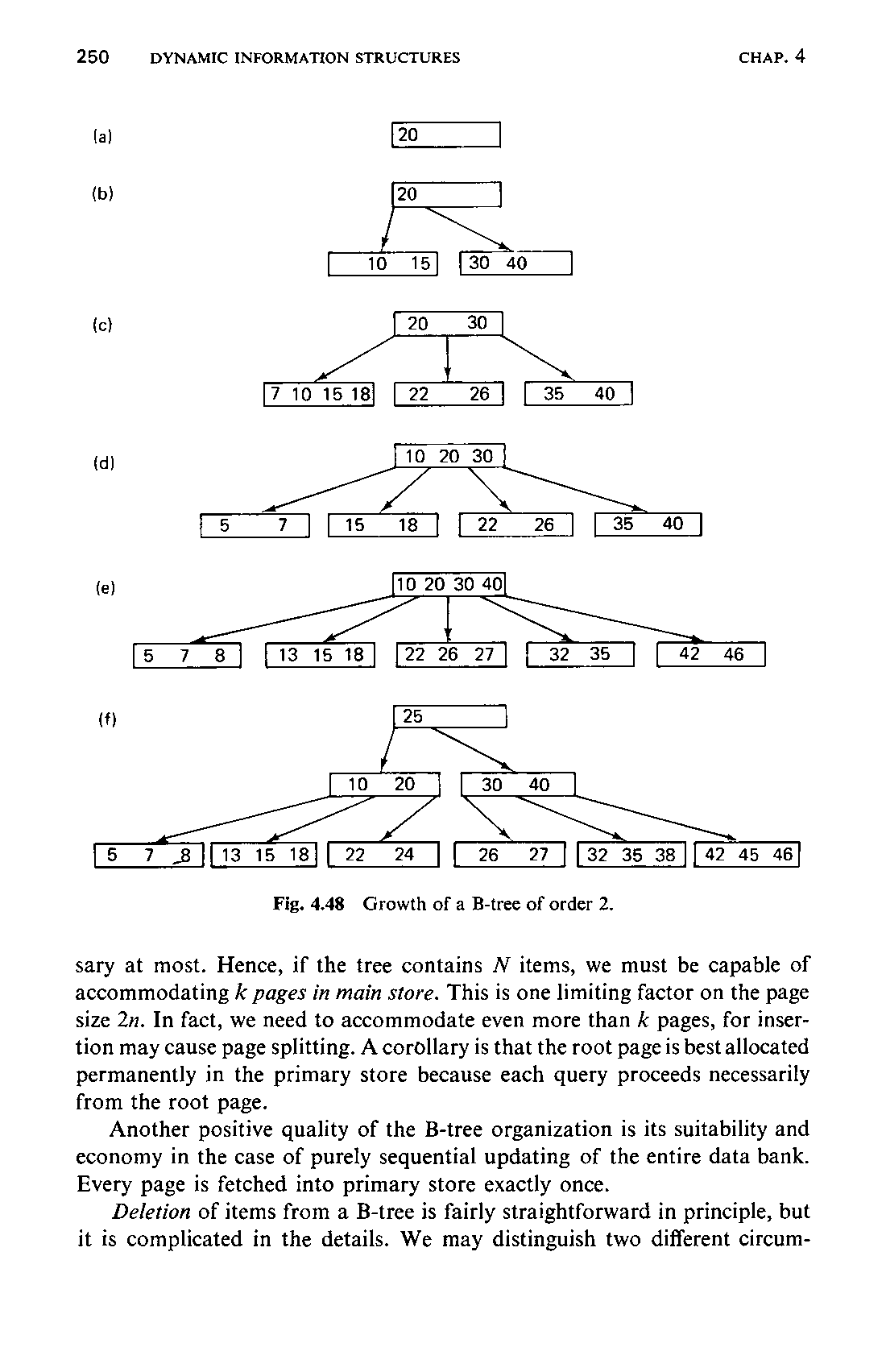
sary at most. Hence, if the tree contains N items, we must be capable of accommodating k pages in main store. This is one limiting factor on the page size 2n. In fact, we need to accommodate even more than k pages, for insertion may cause page splitting. A corollary is that the root page is best allocated permanently in the primary store because each query proceeds necessarily from the root page.

Another positive quality of the B-tree organization is its suitability and economy in the case of purely sequential updating of the entire data bank. Every page is fetched into primary store exactly once.

Deletion of items from a B-tree is fairly straightforward in principle, but it is complicated in the details. We may distinguish two different circum-

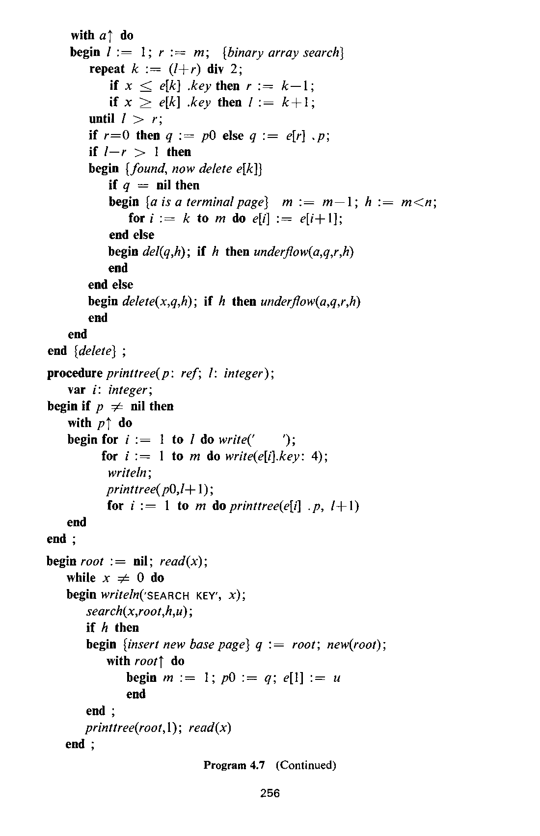
1. The item to be deleted is on a leaf page; here its removal algorithm is plain and simple.

2. The item is not on a leaf page; it must be replaced by one of the two lexicographically adjacent items, which happen to be on leaf pages and can easily be deleted.

In case 2 finding the adjacent key is analogous to finding the one used in binary tree deletion. We descend along the rightmost pointers down to the leaf page P, replace the item to be deleted by the rightmost item on P, and then reduce the size of P by 1.

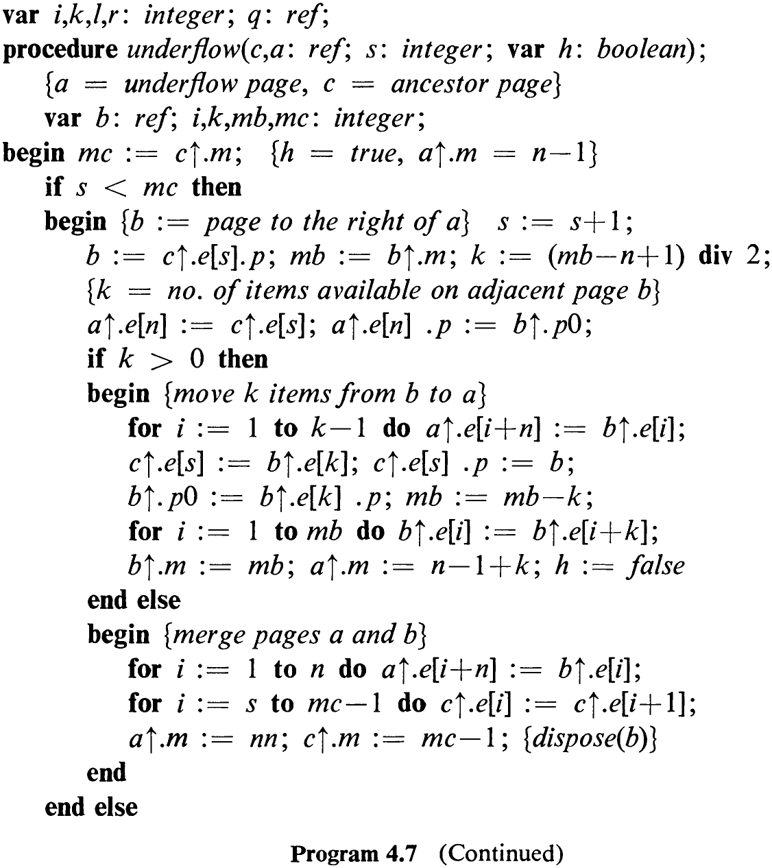
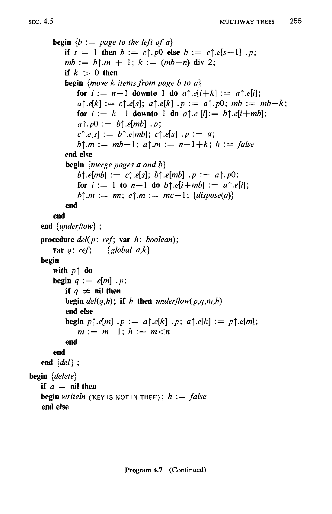
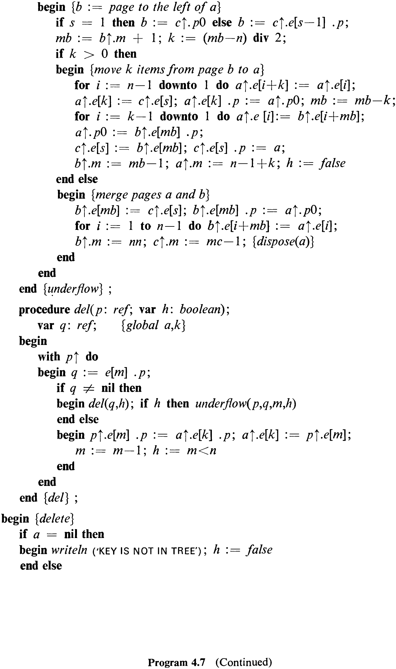
In any case, reduction of size must be followed by a check of the number of items m on the reduced page. For if m <n, the primary characteristic of B-trees would be violated. Some additional action has to be taken; this underflow condition is indicated by the Boolean variable parameter h.

The only recourse is to borrow, or to “annect,” an item from one of the neighboring pages. Since this involves fetching page Q into main store—a relatively costly operation—one is tempted to make the best of this undesirable situation and to annect more than a single item at once. The usual strategy is to distribute the items on pages P and Q evenly on both pages. This is called balancing.

Of course, it may happen that there is no item left to be annected since Q has already reached its minimal size n. In this case the total number of items on pages P and Q is 2n — 1; we may merge the two pages into one, adding the middle item from the ancestor page of P and Q, and then entirely dispose of page Q. This is exactly the inverse process of page splitting. The process may be visualized by considering the deletion of key 22 in Fig. 4.47.

Once again, the removal of the middle key in the ancestor page may cause its size to drop below the permissible limit 1, thereby requiring that further special action (either balancing or merging) be undertaken at the next level. In the extreme case the page merging may propagate all the way up to the root. If the root is reduced to size 0, it is itself deleted, thereby causing a reduction in the height of the B-tree. It is, in fact, the only way that a B-tree may shrink in height.

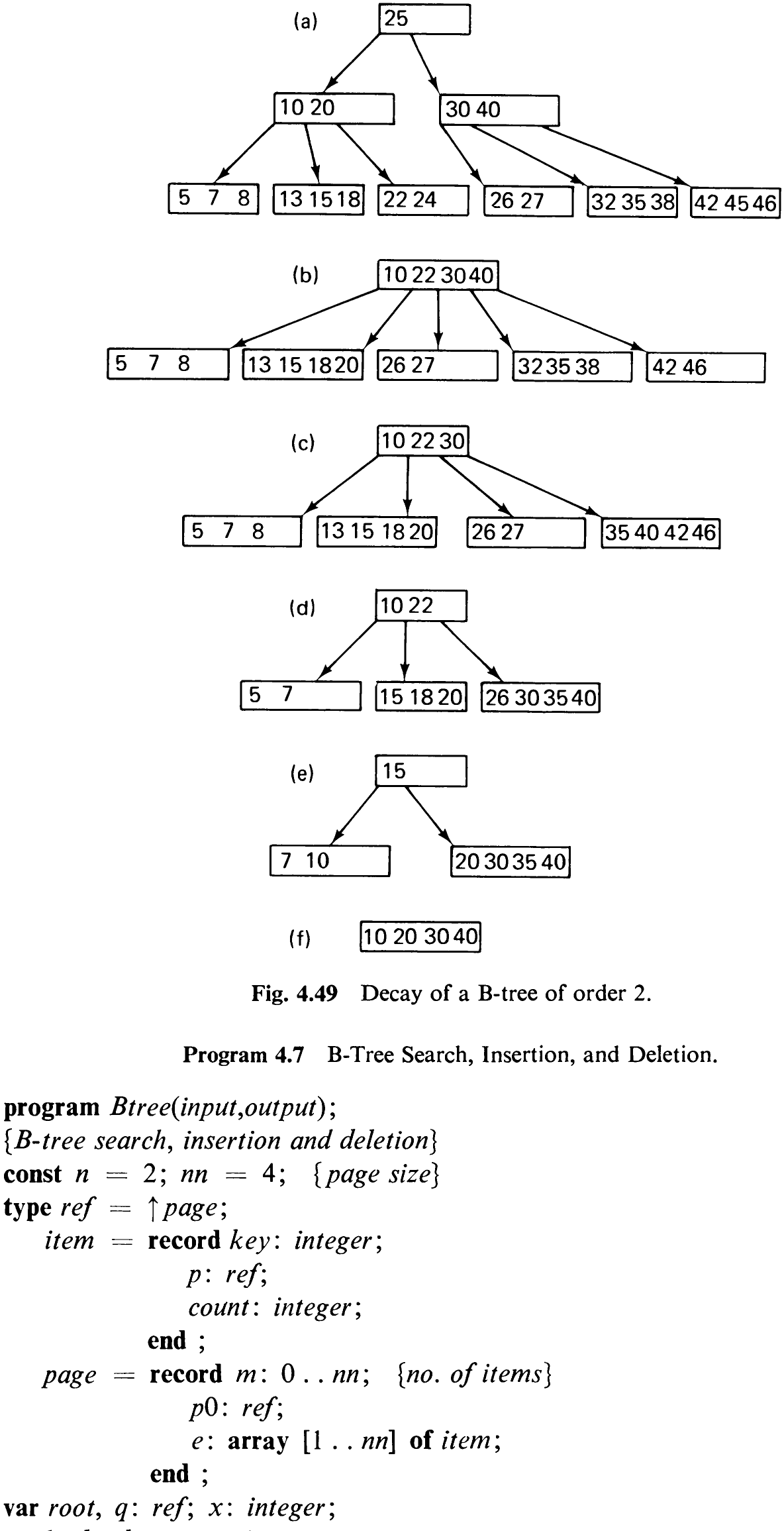
Figure 4.49 shows the gradual decay of the B-tree of Fig. 4.48 upon the sequential deletion of the keys

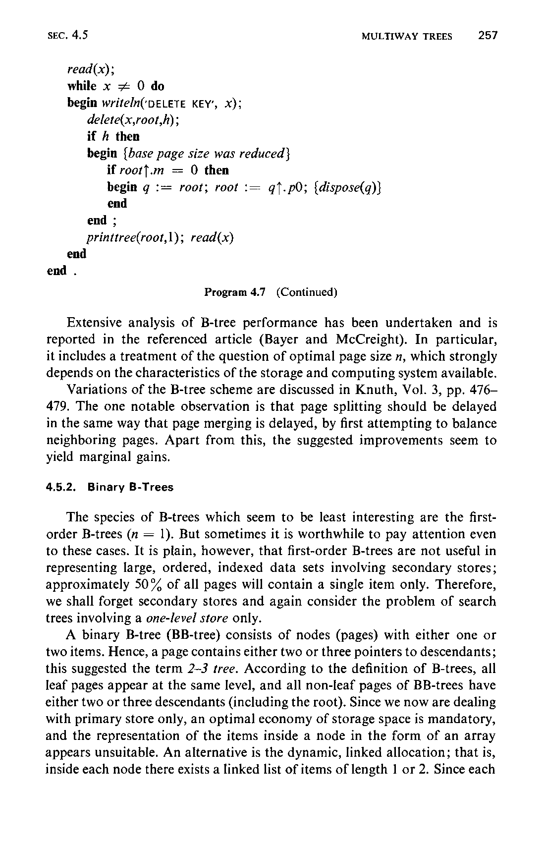
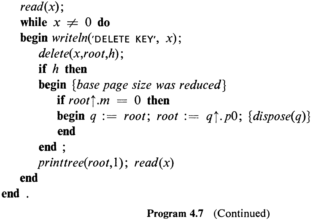
The semicolons again designate the places where the “snapshots” are taken, namely, where pages are being disposed. The deletion algorithm is included as a procedure in Program 4.7. The similarity of its structure to that of balanced tree deletion is particularly noteworthy.

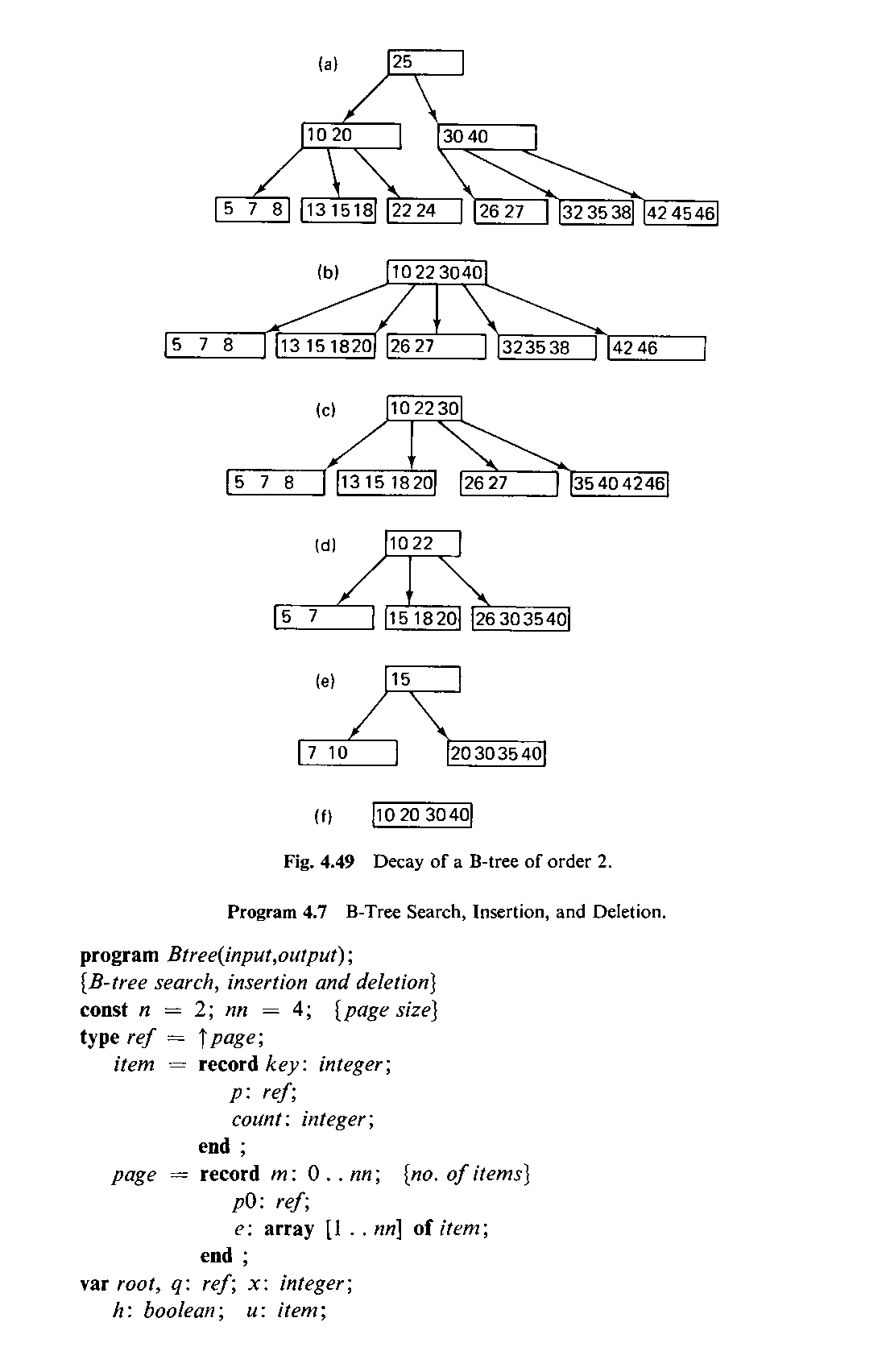
procedure search(x: integer; a: ref; var h: boolean; var v: item); {Search key x on B-tree with root a; if found, increment counter.

otherwise insert an item with key x and count | in tree. If an item emerges to be passed to a lower level, then assign it to v;

{search and delete key x in b-tree a; if a page underflow is

necessary, balance with adjacent page if possible, otherwise merge; h := “page a is undersize”}

Extensive analysis of B-tree performance has been undertaken and is reported in the referenced article (Bayer and McCreight). In particular, it includes a treatment of the question of optimal page size n, which strongly depends on the characteristics of the storage and computing system available.

Variations of the B-tree scheme are discussed in Knuth, Vol. 3, pp. 476- 479. The one notable observation is that page splitting should be delayed in the same way that page merging is delayed, by first attempting to balance neighboring pages. Apart from this, the suggested improvements seem to yield marginal gains.

4.5.2 Binary B-Trees

The species of B-trees which seem to be least interesting are the first-order B-trees (n = 1). But sometimes it is worthwhile to pay attention even to these cases. It is plain, however, that first-order B-trees are not useful in representing large, ordered, indexed data sets involving secondary stores; approximately 50% of all pages will contain a single item only. Therefore, we shall forget secondary stores and again consider the problem of search trees involving a one-level store only.

A binary B-tree (BB-tree) consists of nodes (pages) with either one or two items. Hence, a page contains either two or three pointers to descendants; this suggested the term 2-3 tree. According to the definition of B-trees, all leaf pages appear at the same level, and all non-leaf pages of BB-trees have either two or three descendants (including the root). Since we now are dealing with primary store only, an optimal economy of storage space is mandatory, and the representation of the items inside a node in the form of an array appears unsuitable. An alternative is the dynamic, linked allocation; that is, inside each node there exists a linked list of items of length 1 or 2. Since each

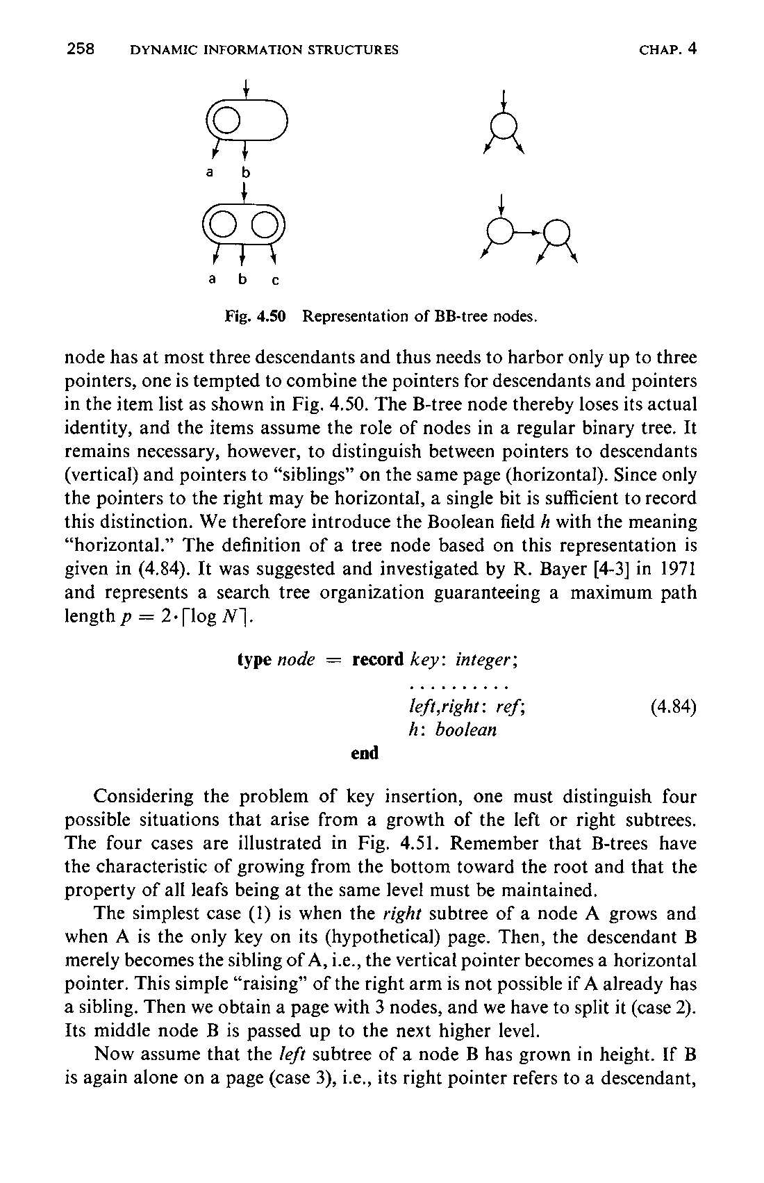
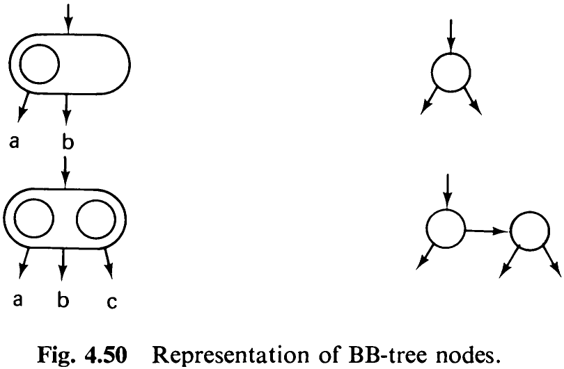
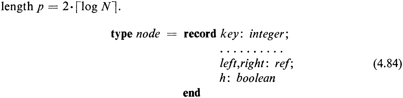
node has at most three descendants and thus needs to harbor only up to three pointers, one is tempted to combine the pointers for descendants and pointers in the item list as shown in Fig. 4.50. The B-tree node thereby loses its actual identity, and the items assume the role of nodes in a regular binary tree. It remains necessary, however, to distinguish between pointers to descendants (vertical) and pointers to “siblings” on the same page (horizontal). Since only the pointers to the right may be horizontal, a single bit is sufficient to record this distinction. We therefore introduce the Boolean field A with the meaning “horizontal.” The definition of a tree node based on this representation is given in (4.84). It was suggested and investigated by R. Bayer [4-3] in 1971 and represents a search tree organization guaranteeing a maximum path

Considering the problem of key insertion, one must distinguish four possible situations that arise from a growth of the left or right subtrees. The four cases are illustrated in Fig. 4.51. Remember that B-trees have the characteristic of growing from the bottom toward the root and that the property of all leafs being at the same level must be maintained.

The simplest case (1) is when the right subtree of a node A grows and when A is the only key on its (hypothetical) page. Then, the descendant B merely becomes the sibling of A, i.e., the vertical pointer becomes a horizontal pointer. This simple “raising” of the right arm is not possible if A already has a sibling. Then we obtain a page with 3 nodes, and we have to split it (case 2). Its middle node B is passed up to the next higher level.

Now assume that the /eft subtree of a node B has grown in height. If B is again alone on a page (case 3), i.e., its right pointer refers to a descendant,

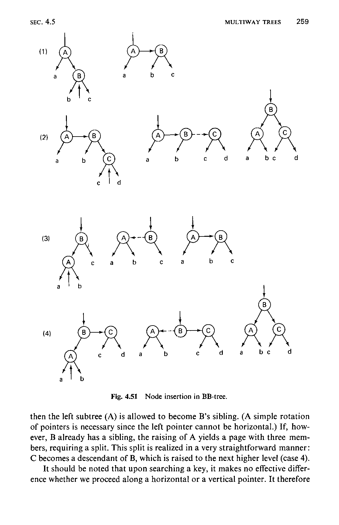
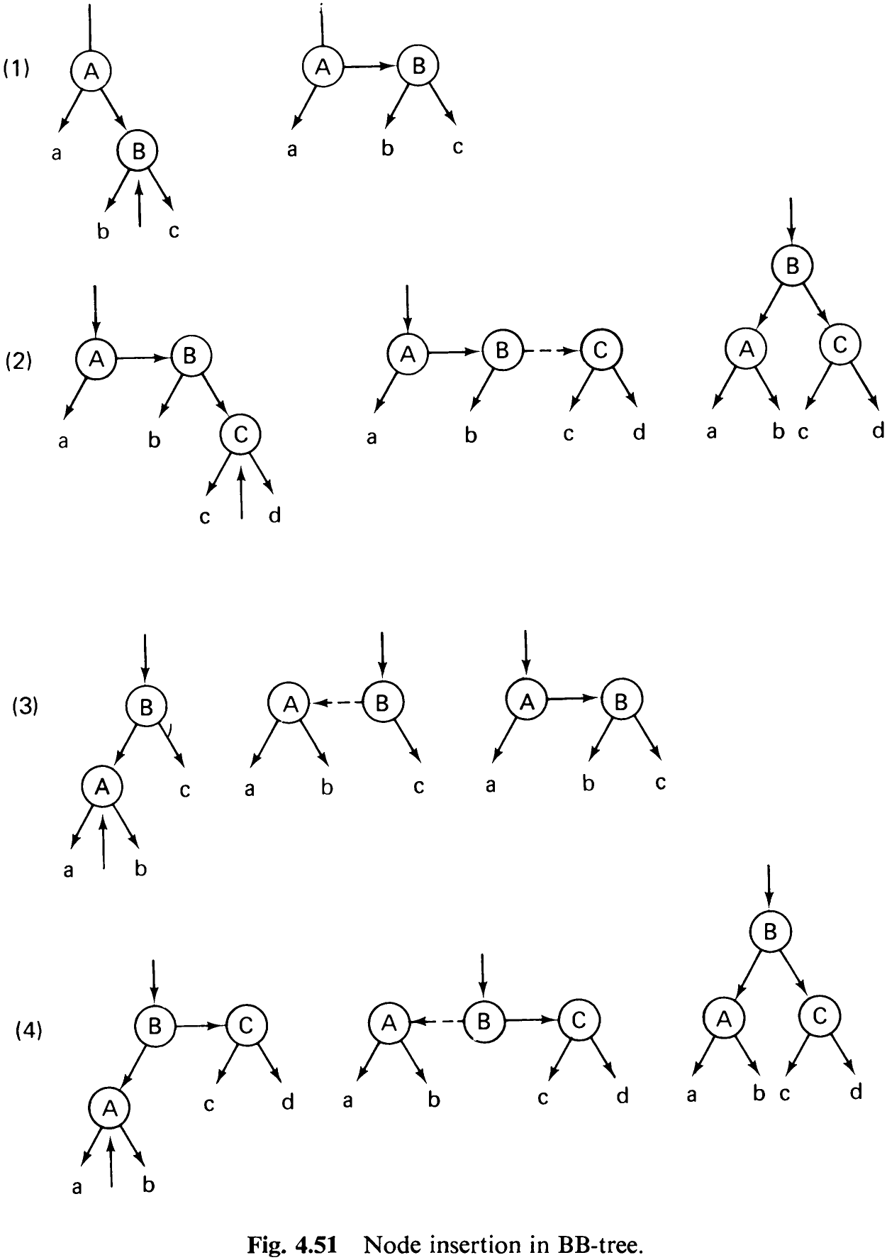
then the left subtree (A) is allowed to become B’s sibling. (A simple rotation of pointers is necessary since the left pointer cannot be horizontal.) If, however, B already has a sibling, the raising of A yields a page with three members, requiring a split. This split is realized in a very straightforward manner: C becomes a descendant of B, which is raised to the next higher level (case 4).

It should be noted that upon searching a key, it makes no effective difference whether we proceed along a horizontal or a vertical pointer. It therefore260 appears artificial to worry about a left pointer in case 3 becoming horizontal, although its page still contains not more than two members. Indeed, the insertion algorithm reveals a strange asymmetry in handling the growth of left and right subtrees, and it lets the BB-tree organization appear rather artificial. There is no “proof” of strangeness of this organization; yet a healthy intuition tells us that something is “fishy” and that we should remove this asymmetry. It leads to the notion of the symmetric binary B-tree(SBB-tree) which was also investigated by Bayer [4-4] in 1972. On the average it leads to slightly more efficient search trees, but the algorithms for insertion and deletion are also slightly more complex. Moreover, each node now requires two bits (Boolean variables /h and rh) to indicate the nature of its two pointers.

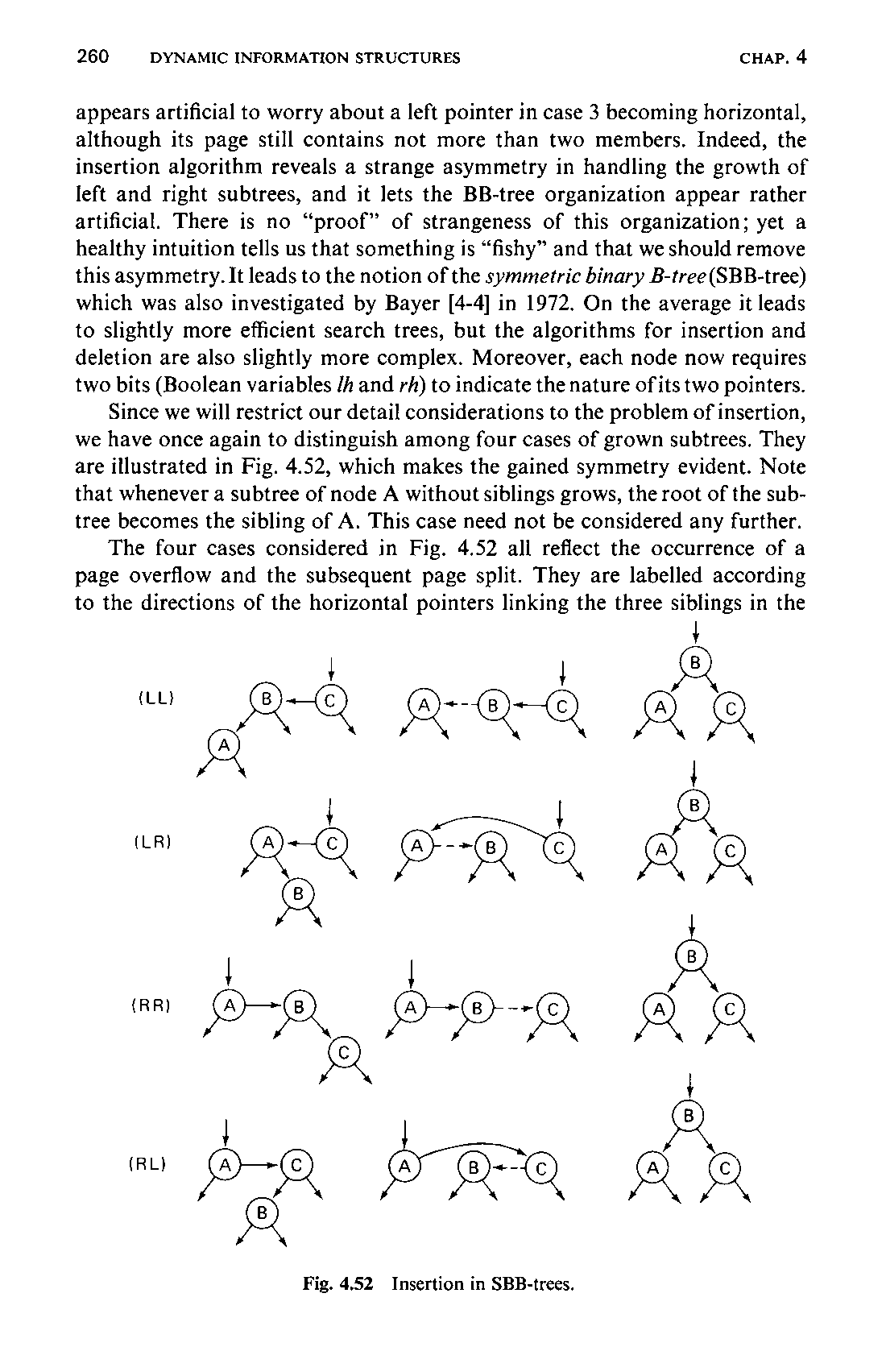
Since we will restrict our detail considerations to the problem of insertion, we have once again to distinguish among four cases of grown subtrees. They are illustrated in Fig. 4.52, which makes the gained symmetry evident. Note that whenever a subtree of node A without siblings grows, the root of the subtree becomes the sibling of A. This case need not be considered any further.

The four cases considered in Fig. 4.52 all reflect the occurrence of a page overflow and the subsequent page split. They are labelled according to the directions of the horizontal pointers linking the three siblings in the

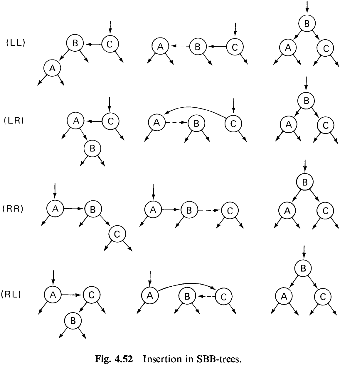
middle figures. The initial situation is shown in the left column; the middle column illustrates the fact that the lower node has been raised as its subtree has grown; the figures in the right column show the result of node re-arrangement (page split).

It is advisable to stick no longer to the notion of pages out of which this organization had developed, for all we are interested in is to bound the maximum path length to 2-log N. For this we need only to ensure that nowhere are there two successive horizontal pointers on any search path. However, there is no reason to forbid any nodes with horizontal pointers to the left and right. We will therefore define the SBB-tree as a tree that has the following properties:

1. Every node contains one key and at most two (pointers to) subtrees.

2. Every pointer is either horizontal or vertical. There are no two consecutive horizontal pointers on any search path.

3. All terminal nodes (nodes without descendants) appear at the same (terminal) level.

From this definition it follows that the longest search path is no longer than twice the height of the tree. Since no SBB-tree with N nodes can have a height larger than [log N |, it follows immediately that 2[ log N | is an upper bound on the search path length.

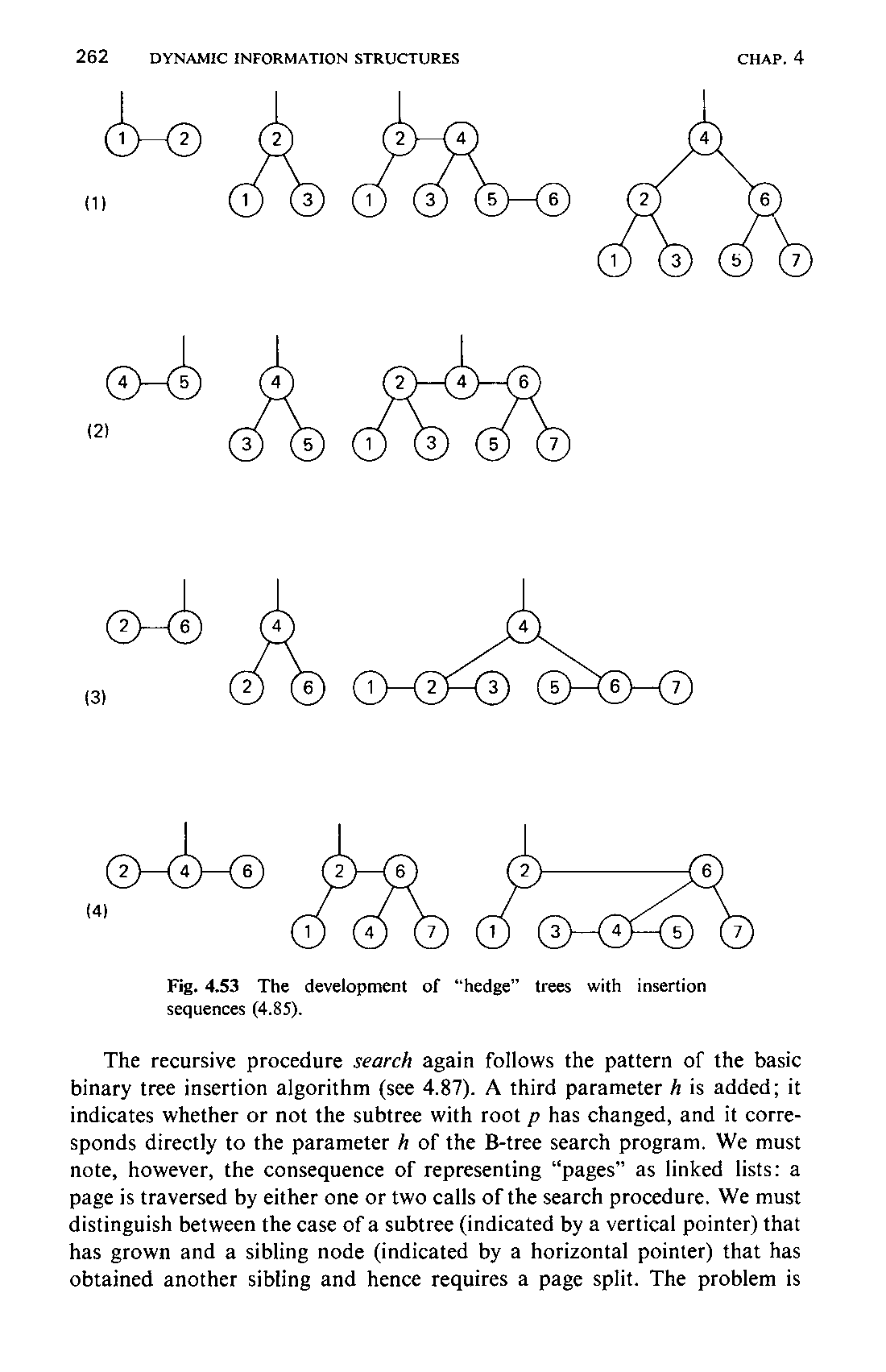
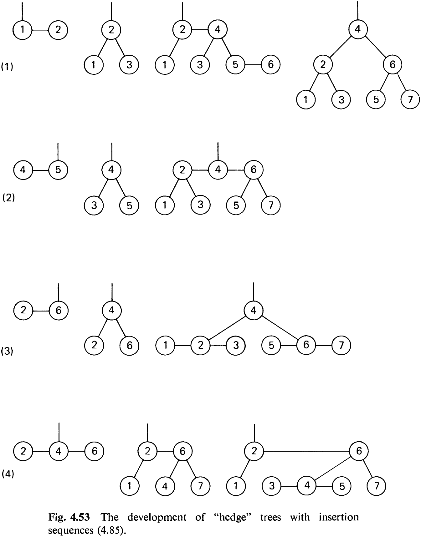
In order to let the reader visualize how these trees grow, he is referred to Fig. 4.53. The lines represent snapshots taken during the insertion of the following sequences of keys, where every semicolon marks a snapshot.

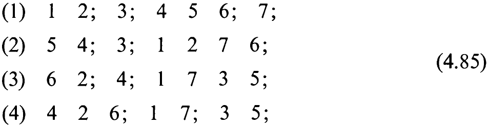
These pictures make the third property of B-trees particularly obvious: all terminal nodes appear on the same level. One is therefore inclined to compare these structures with garden hedges that have been recently trimmed with hedge scissors. We call these structures hedges.

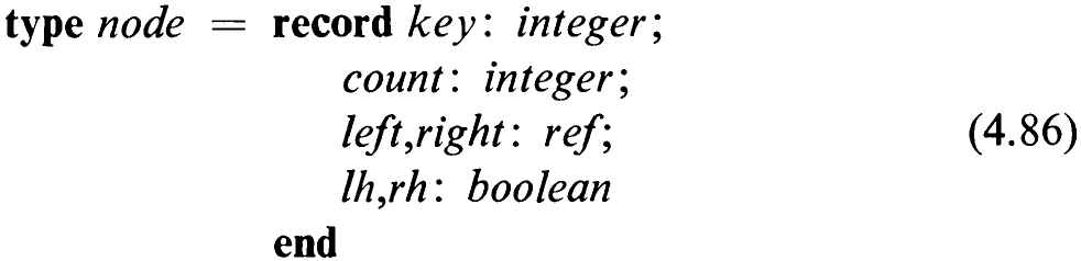
The algorithm for the construction of hedge-trees is formulated in (4.87). It is based on a definition of the node type (4.86) with the two components /h and rh denoting horizontality of the left and right pointers.

The recursive procedure search again follows the pattern of the basic binary tree insertion algorithm (see 4.87). A third parameter / is added; it indicates whether or not the subtree with root p has changed, and it corresponds directly to the parameter /# of the B-tree search program. We must note, however, the consequence of representing “pages” as linked lists: a page is traversed by either one or two calls of the search procedure. We must distinguish between the case of a subtree (indicated by a vertical pointer) that has grown and a sibling node (indicated by a horizontal pointer) that has obtained another sibling and hence requires a page split. The problem is263 easily solved by introducing a three-valued A with the following meanings:

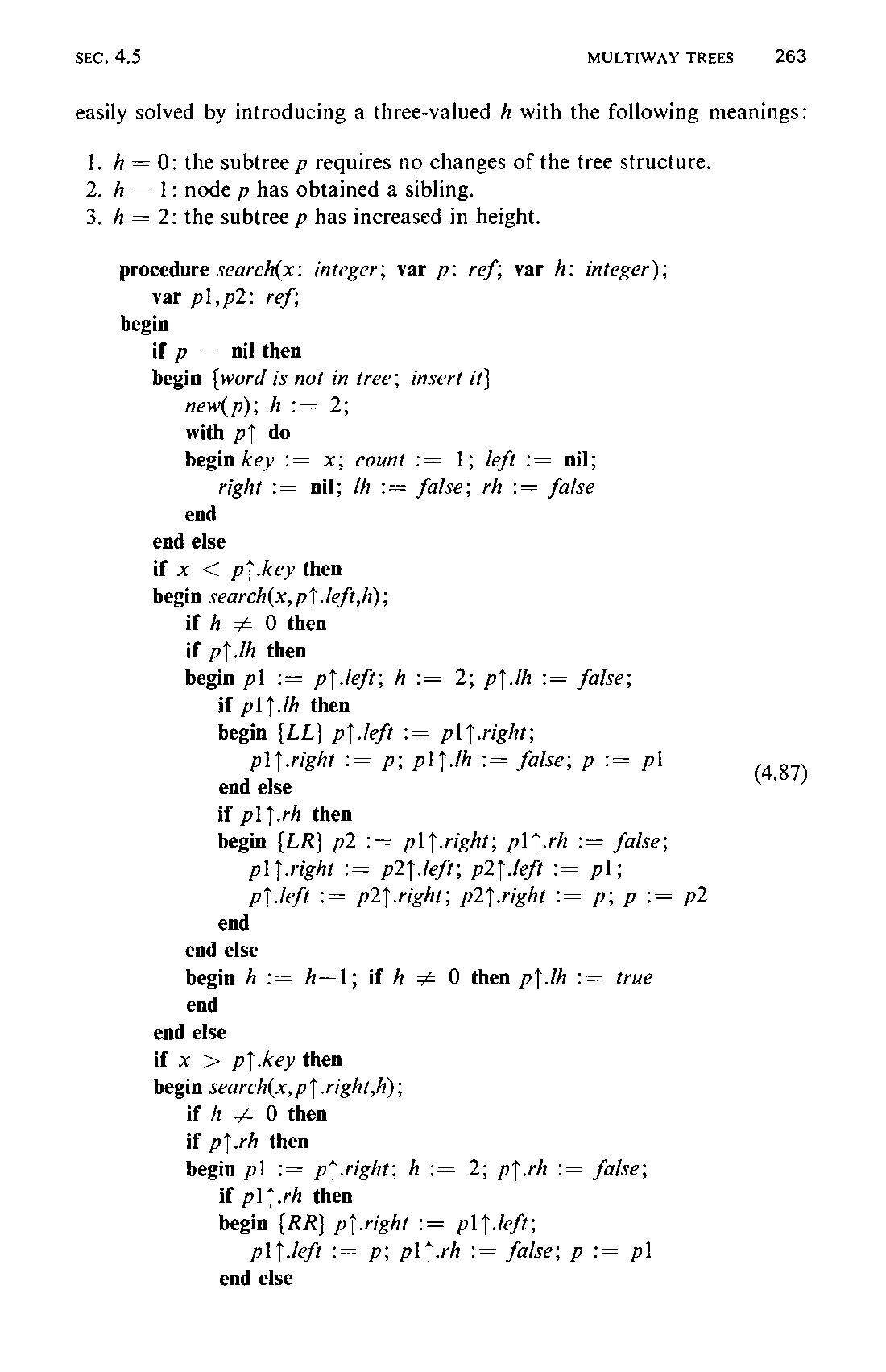
1. h = 0: the subtree p requires no changes of the tree structure.

2. h = 1: node p has obtained a sibling.

3. h = 2: the subtree p has increased in height.

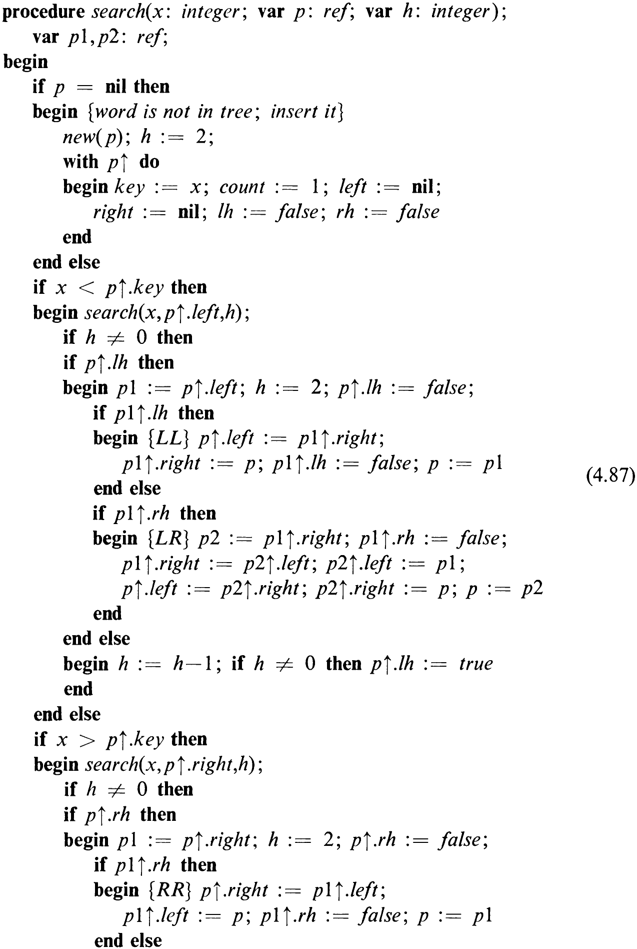
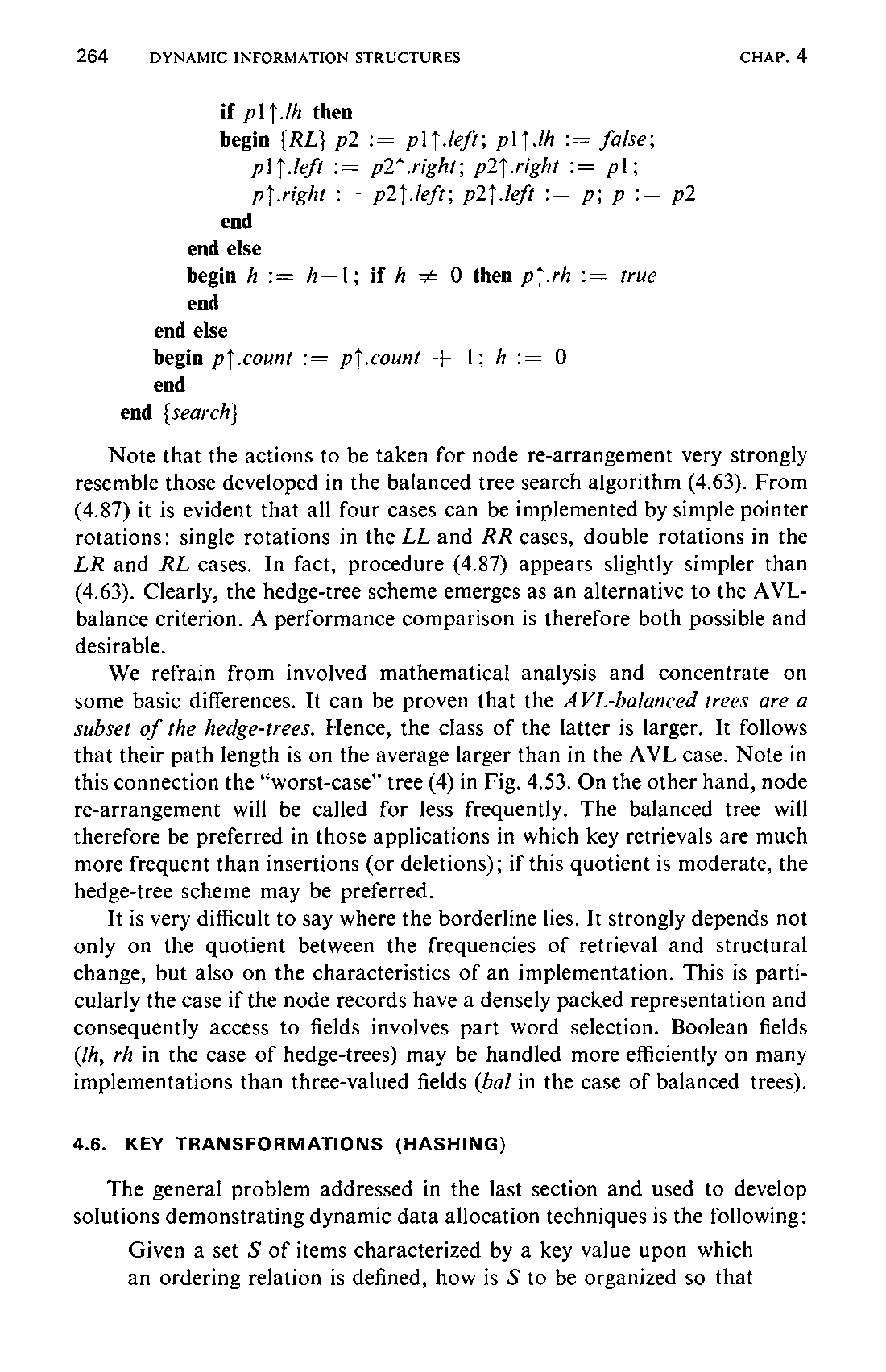
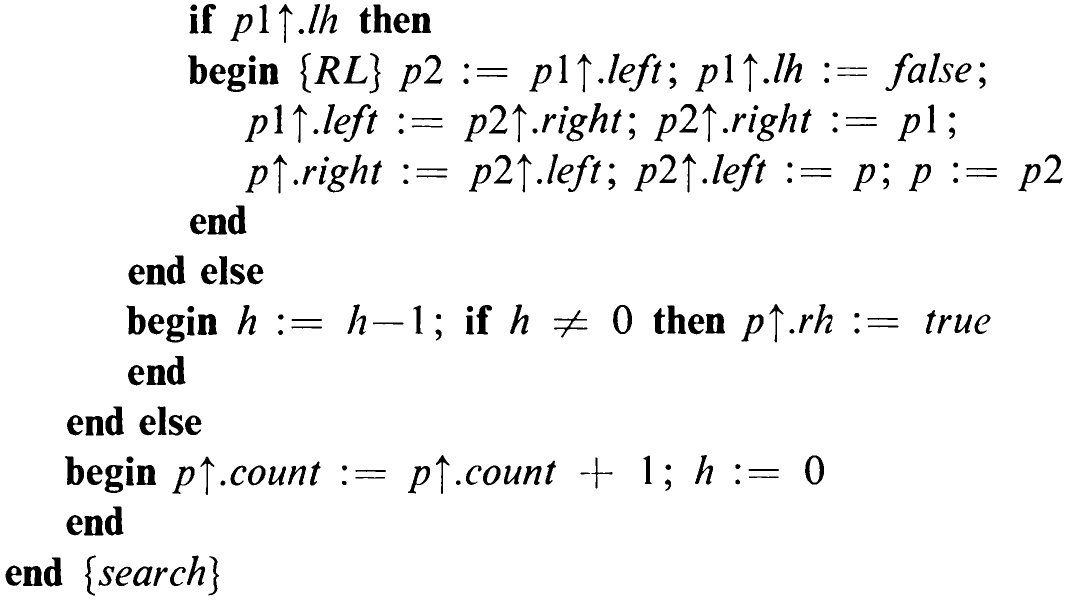
Note that the actions to be taken for node re-arrangement very strongly resemble those developed in the balanced tree search algorithm (4.63). From (4.87) it is evident that all four cases can be implemented by simple pointer rotations: single rotations in the LL and RR cases, double rotations in the LR and RL cases. In fact, procedure (4.87) appears slightly simpler than (4.63). Clearly, the hedge-tree scheme emerges as an alternative to the AVLbalance criterion. A performance comparison is therefore both possible and desirable.

We refrain from involved mathematical analysis and concentrate on some basic differences. It can be proven that the AVL-balanced trees are a subset of the hedge-trees. Hence, the class of the latter is larger. It follows that their path length is on the average larger than in the AVL case. Note in this connection the “worst-case” tree (4) in Fig. 4.53. On the other hand, node re-arrangement will be called for less frequently. The balanced tree will therefore be preferred in those applications in which key retrievals are much more frequent than insertions (or deletions); if this quotient is moderate, the hedge-tree scheme may be preferred.

It is very difficult to say where the borderline lies. It strongly depends not only on the quotient between the frequencies of retrieval and structural change, but also on the characteristics of an implementation. This is particularly the case if the node records have a densely packed representation and consequently access to fields involves part word selection. Boolean fields (Jh, rh in the case of hedge-trees) may be handled more efficiently on many implementations than three-valued fields (ba/ in the case of balanced trees).