Key Transformations (Hashing)

The general problem addressed in the last section and used to develop solutions demonstrating dynamic data allocation techniques is the following:

Clearly, in a computer store each item is ultimately accessed by specifying a storage address a. Hence, the stated problem is essentially one of finding an appropriate mapping H of keys (K) into addresses (A):

In Sect. 4.5 this mapping was implemented in the form of various list and tree search algorithms based on different underlying data organizations. Here we present yet another approach that is basically simple and very efficient in many cases. The fact that it also has some disadvantages will be discussed subsequently.

The data organization used in this technique is the array structure. H is therefore a mapping transforming keys into array indices, which is the reason for the term key transformation that is generally used for this technique. It should be noted that we shall not need to rely on any dynamic allocation procedures because the array is one of the fundamental, static structures. This paragraph is thus somewhat misplaced under the chapter heading of dynamic information structures, but since it is often used in problem areas where tree structures are comparable competitors, this seems to be an appropriate place for its presentation.

The fundamental difficulty in using a key transformation is that the set of possible key values is very much larger than the set of available store addresses (array indices). A typical example is the use of alphabetical words with, say, up to 10 letters as keys for the identification of individuals in a set of, say, up to a thousand persons. Hence, there are 26!° possible keys, which are to be mapped onto 10? possible indices. The function H is therefore obviously a many-to-one function. Given a key k, the first step in a retrieval (search) operation is to compute its associated index h = H(k), and the second —evidently necessary—step is to verify whether or not the item with the key k is indeed identified by A in the array (table) 7, i.e., to check whether T[H(k)].key = k. We are immediately confronted with two questions:

1. What kind of function H should be used?

2. How do we cope with the situation that H does not yield the location of the desired item?

The answer to question 2 is that some method must be used to yield an alternative location, say index h’, and, if this is still not the location of the wanted item, yet a third index 4”, and so on. The case in which a key other than the desired one is at the identified location is called a collision; the task of generating alternative indices is termed collision handling. In the following we shall discuss the choice of a transformation function and methods of collision handling.

4.6.1 Choice of a Transformation Function

A prerequisite of a good transformation function is that it distributes the keys as evenly as possible over the range of index values. Apart from satisfying this requirement, the distribution is not bound to any pattern, and it is actually desirable if it gives the impression that it is entirely at random. This property has given this method the somewhat unscientific name hashing, i.e., “chopping the argument up” or “making a mess,” and H is called the hash function. Clearly, it should be efficiently computable, i.e., be composed of very few basic arithmetic operations.

Assume that a transfer function ord(k) is available and denotes the ordinal number of the key & in the set of all possible keys. Assume, furthermore, that the array indices i range over the integers 0... N — 1, where N is the size of the array. Then an obvious choice is

It has the property that the key values are spread evenly over the index range, and it is therefore the basis of most key transformations. It is also extremely efficiently computable if N is a power of 2. But it is exactly this case that must be avoided if the keys are sequences of letters. The assumption that all keys are equally likely is in this case entirely erroneous. In fact, words which differ by only a few characters will then most likely map onto identical indices, thus effectively causing a most uneven distribution. In (4.88) it is therefore particularly recommended to let N be a prime number [4-7]. This has the consequence that a full division operation is needed that cannot be replaced by a mere masking of binary digits, but this is no serious drawback on most modern computers that feature a built-in division instruction.

Often, hash functions are used which consist of applying logical operations such as the “exclusive or” to some parts of the key represented as a sequence of binary digits. These operations may be faster than division on some computers, but they sometimes fail spectacularly to distribute the keys evenly over the range of indices. We therefore refrain from discussing such methods in further detail.

4.6.2 Collision Handling

If an entry in the table corresponding to a given key turns out to be not the desired item, then a collision is present, i.e., two items have keys mapping onto the same index. A second probe is necessary, one based on an index obtained in a deterministic manner from the given key. There exist several methods of generating secondary indices. An obvious and effective one is linking all entries with identical primary index H(k) together as a linked list. This is called direct chaining. The elements of this list may either be in the267 primary table or not; in the latter case, storage in which they are allocated is usually called an overflow area. This method is quite effective, although it has the disadvantage that secondary lists must be maintained and that each entry must provide space for a pointer (or index) to its list of collided items.

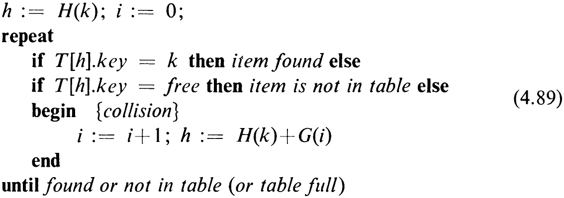
An alternative solution for resolving collisions is to dispense with links entirely and instead simply look at other entries in the same table until the item is found or an open position is encountered, in which case one may assume that the specified key is not present in the table. This method is called open addressing [4-9]. Naturally, the sequence of indices of secondary probes must always be the same for a given key. The algorithm for a table lookup can then be sketched as follows:

Various functions for resolving collisions have been proposed in the literature. A survey of the topic by Morris in 1968 [4-8] stimulated considerable activities in this field. The simplest method is to try for the next location —considering the table to be circular—until either the item with the specified key is found or an empty location is encountered. Hence, G(i) = i; the indices h, used for probing in this case are

This method is called linear probing and has the disadvantage that entries have a tendency to cluster around the primary keys (keys that had not collided upon insertion). Ideally, of course, a function G should be chosen which again spreads the keys uniformly over the remaining set of locations. In practice, however, this tends to be too costly, and methods which offer a compromise by being simple to compute and still superior to the linear function (4.90) are preferred. One of them consists of using a quadratic function such that the sequence of indices for probing is

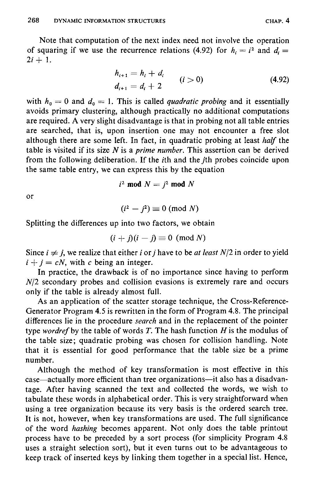
Note that computation of the next index need not involve the operation of squaring if we use the recurrence relations (4.92) for h,; = i? and d, =

with h, = 0 and d, = 1. This is called quadratic probing and it essentially avoids primary clustering, although practically no additional computations are required. A very slight disadvantage is that in probing not all table entries are searched, that is, upon insertion one may not encounter a free slot although there are some left. In fact, in quadratic probing at least half the table is visited if its size N is a prime number. This assertion can be derived from the following deliberation. If the ith and the jth probes coincide upon the same table entry, we can express this by the equation

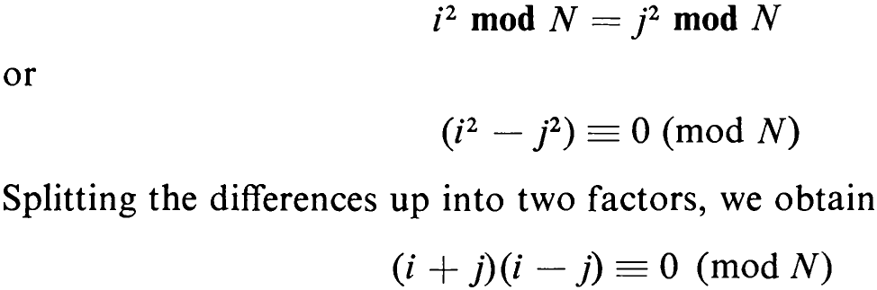
Since i + j, we realize that either i or j have to be at least N/2 in order to yield i+ j= cN, with c being an integer.

In practice, the drawback is of no importance since having to perform N/2 secondary probes and collision evasions is extremely rare and occurs only if the table is already almost full.

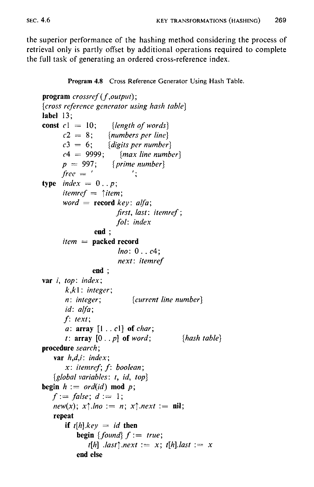
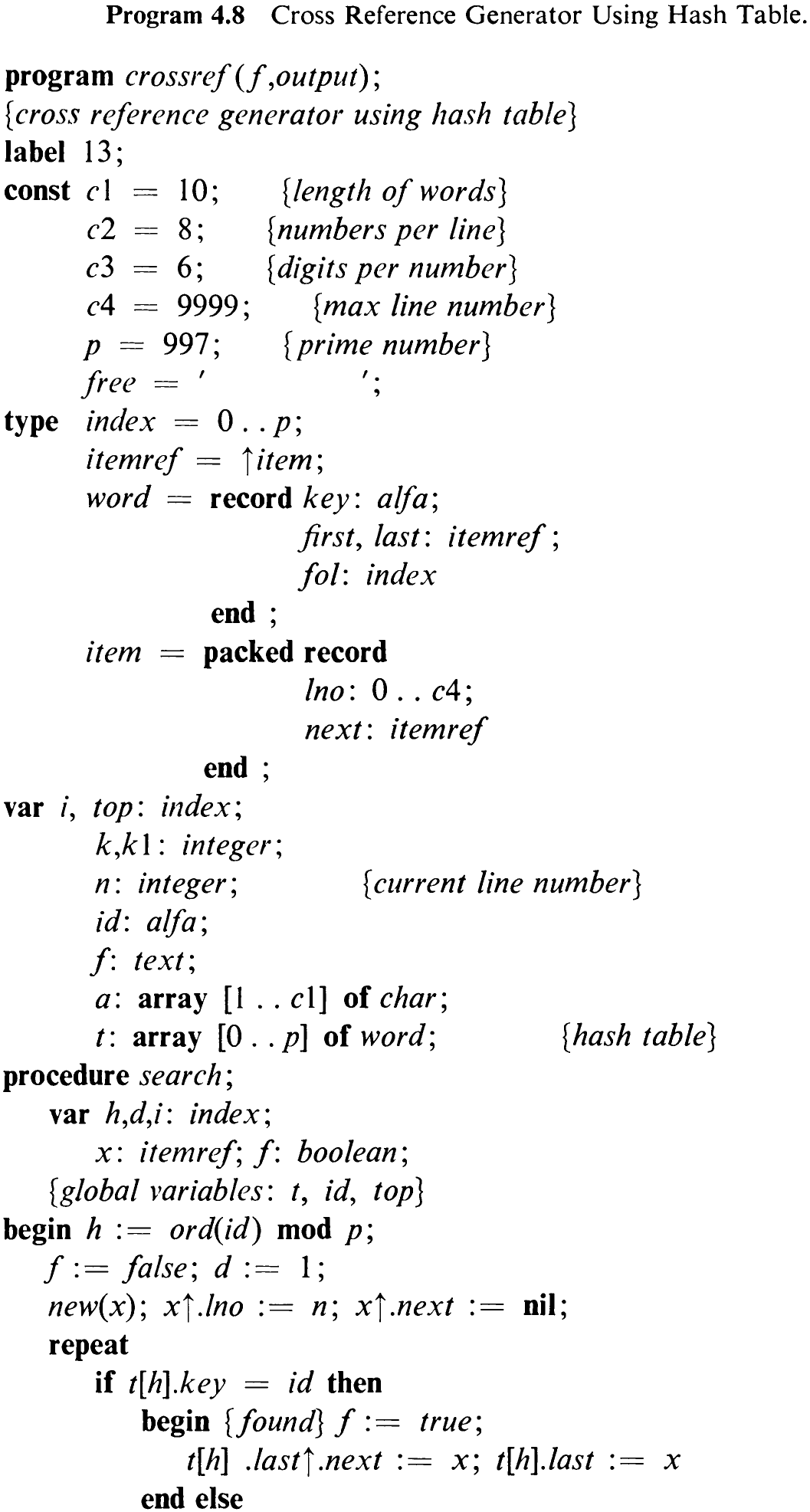
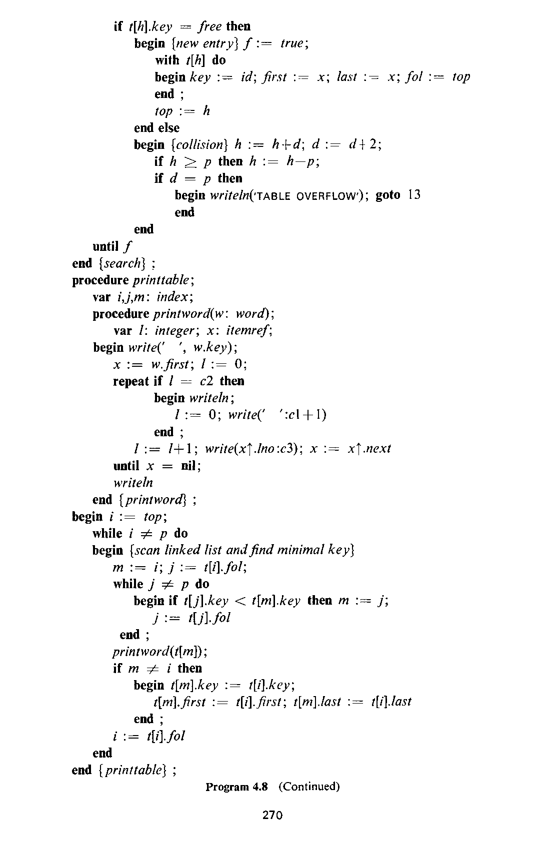
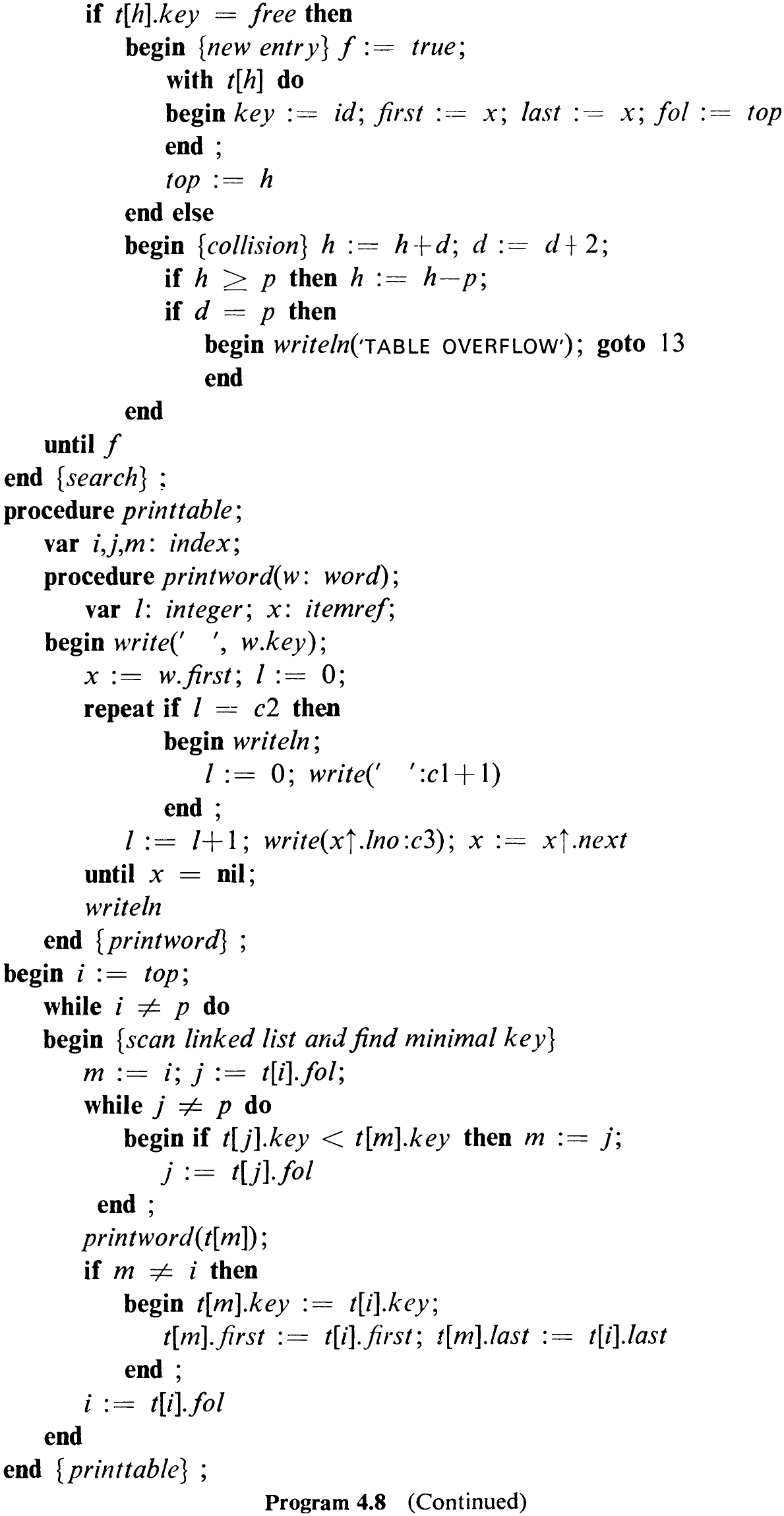
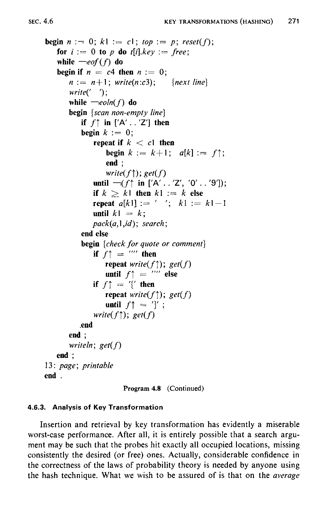
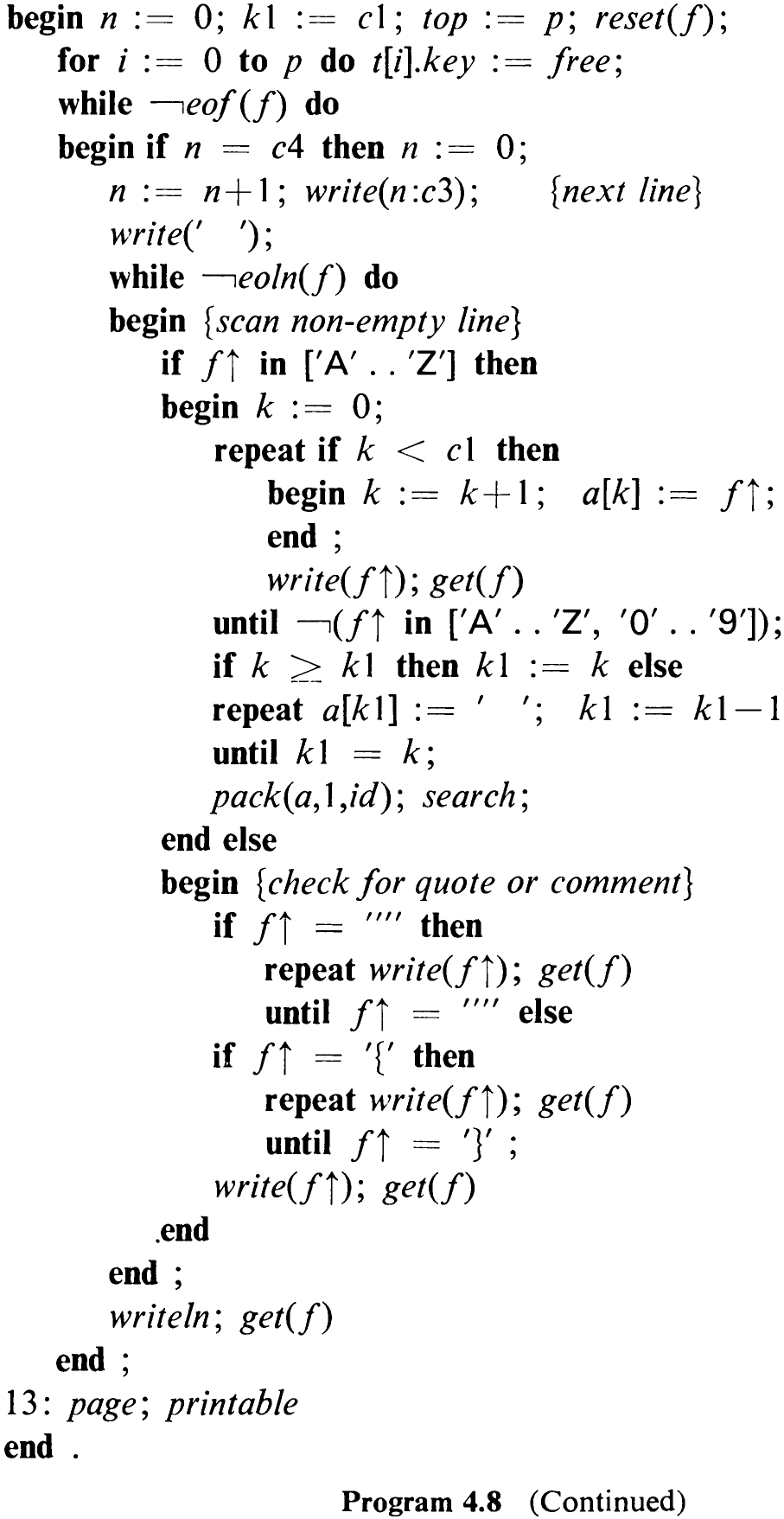
As an application of the scatter storage technique, the Cross-ReferenceGenerator Program 4.5 is rewritten in the form of Program 4.8. The principal differences lie in the procedure search and in the replacement of the pointer type wordref by the table of words 7. The hash function H is the modulus of the table size; quadratic probing was chosen for collision handling. Note that it is essential for good performance that the table size be a prime number.

Although the method of key transformation is most effective in this case—actually more efficient than tree organizations—it also has a disadvantage. After having scanned the text and collected the words, we wish to tabulate these words in alphabetical order. This is very straightforward when using a tree organization because its very basis is the ordered search tree. It is not, however, when key transformations are used. The full significance of the word hashing becomes apparent. Not only does the table printout process have to be preceded by a sort process (for simplicity Program 4.8 uses a straight selection sort), but it even turns out to be advantageous to keep track of inserted keys by linking them together in a special list. Hence,269 the superior performance of the hashing method considering the process of retrieval only is partly offset by additional operations required to complete the full task of generating an ordered cross-reference index.

4.6.3 Analysis of Key Transformation

Insertion and retrieval by key transformation has evidently a miserable worst-case performance. After all, it is entirely possible that a search argument may be such that the probes hit exactly all occupied locations, missing consistently the desired (or free) ones. Actually, considerable confidence in the correctness of the laws of probability theory is needed by anyone using the hash technique. What we wish to be assured of is that on the average272 the number of probes is small. The following probabilistic argument reveals that it is even very small.

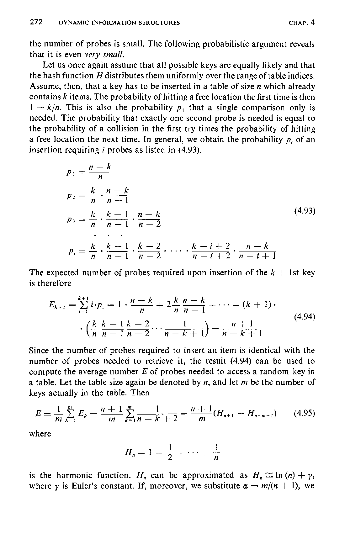
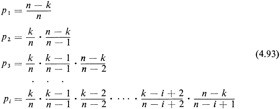
Let us once again assume that all possible keys are equally likely and that the hash function H distributes them uniformly over the range of table indices. Assume, then, that a key has to be inserted in a table of size n which already contains k items. The probability of hitting a free location the first time is then 1 — k/n. This is also the probability p, that a single comparison only is needed. The probability that exactly one second probe is needed is equal to the probability of a collision in the first try times the probability of hitting a free location the next time. In general, we obtain the probability p, of an insertion requiring i probes as listed in (4.93).

The expected number of probes required upon insertion of the k + Ist key is therefore

Since the number of probes required to insert an item is identical with the number of probes needed to retrieve it, the result (4.94) can be used to compute the average number E of probes needed to access a random key in a table. Let the table size again be denoted by n, and let m be the number of keys actually in the table. Then

is the harmonic function. H, can be approximated as H, = In(m) + }, where y is Euler’s constant. If, moreover, we substitute « = m/(n + 1), we

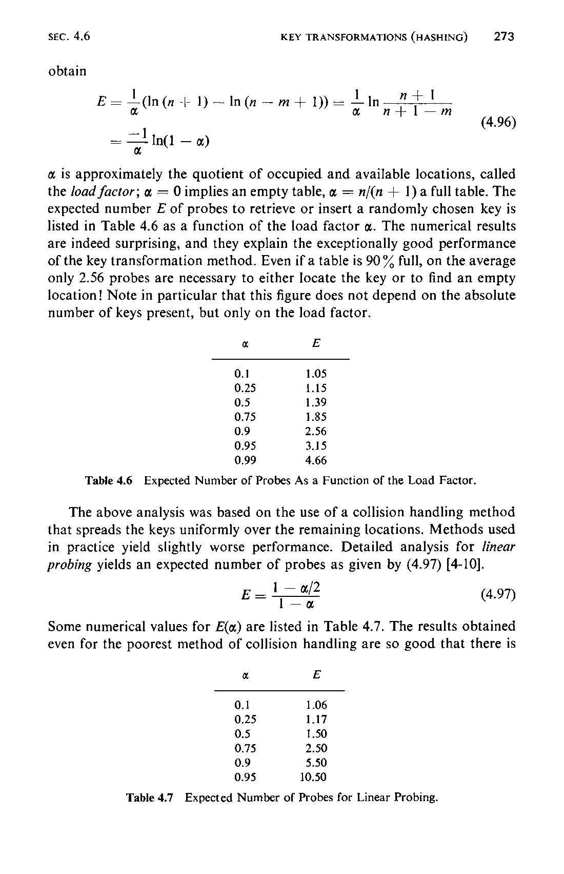
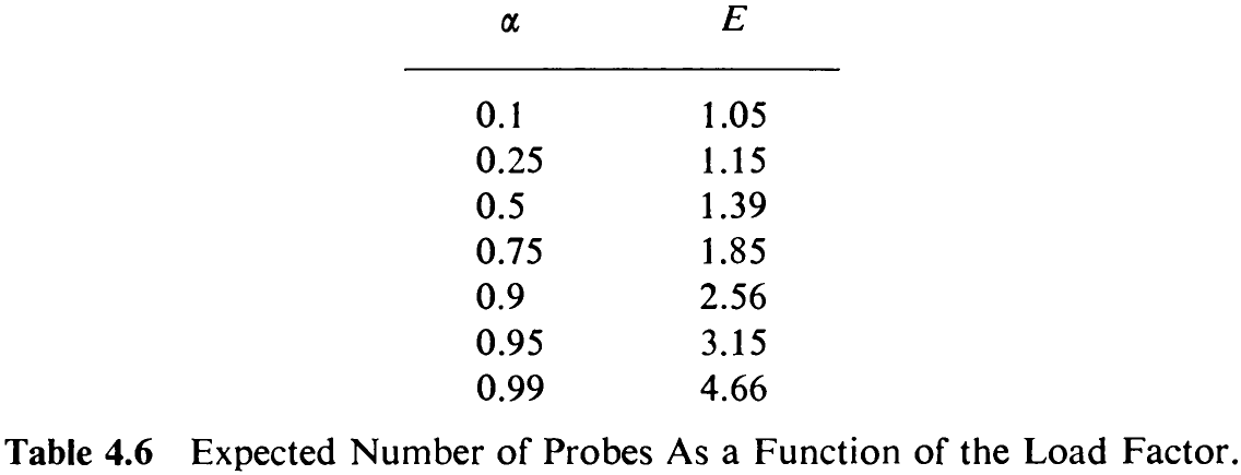
a is approximately the quotient of occupied and available locations, called the load factor; « = 0 implies an empty table, « = n/(n + 1) a full table. The expected number E of probes to retrieve or insert a randomly chosen key is listed in Table 4.6 as a function of the load factor «. The numerical results are indeed surprising, and they explain the exceptionally good performance of the key transformation method. Even if a table is 90 % full, on the average only 2.56 probes are necessary to either locate the key or to find an empty location! Note in particular that this figure does not depend on the absolute number of keys present, but only on the load factor.

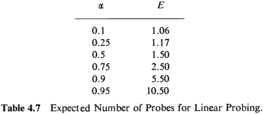
The above analysis was based on the use of a collision handling method that spreads the keys uniformly over the remaining locations. Methods used in practice yield slightly worse performance. Detailed analysis for linear probing yields an expected number of probes as given by (4.97) [4-10].

Some numerical values for E(a) are listed in Table 4.7. The results obtained even for the poorest method of collision handling are so good that there is

a temptation to regard key transformation (hashing) as the panacea for everything. This is particularly so because its performance is superior even to the most sophisticated tree organization discussed, at least on the basis of comparison steps needed for retrieval and insertion. It is therefore important to point out explicitly some of the drawbacks of hashing, even if they are obvious upon unbiased consideration.

Certainly the major disadvantage over techniques using dynamic allocation is that the size of the table is fixed and cannot be adjusted to actual demand. A fairly good a priori estimate of the number of data items to be classified is therefore mandatory if either poor storage utilization or poor performance (or even table overflow) is to be avoided. Even if the number of items is exactly known—an extremely rare case—the desire for good performance dictates to dimension the table slightly (say 10%) too large.

The second major deficiency of scatter storage techniques becomes evident if keys are not only to be inserted and retrieved, but if they are also to be deleted, for deletion of entries in a hash table is extremely cumbersome unless direct chaining in a separate overflow area is used. It is thus fair to say that tree organizations are still attractive, and actually to be preferred, if the volume of data is largely unknown, is strongly variable, and at times even decreases.